KEMM37 Lab 1B - SANS Data Analysis using SasView

Table of Contents
4. Rapid Evaluation of SANS data
4.1 Background Information
4.2 Evaluation of the SANS data
. 4.3 Guiner and Kratky Plots

5. Rapid Evaluation of SANS data

This part of the exercise will use the same real SANS data as the last exercise - taken from a study of surfactant self assembly in deep eutectic solvents (DES).

If you are continuing directly from the first part of the exercise - "Familiarisation with SasView? and Data Handling" you can skip to TASK 17, otherwise start with TASK 10.

TASK 10: Restart SasView

Before starting this part of the exercise, you should have a clean SasView instance. Quit SasView and restart it.

4.1 Background Information

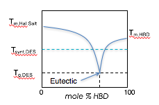
Deep eutectic solvents are a class of ionic liquids formed from a hydrogen bond donor and a halide salt. At a certain mixture ratio, the eutectic mixture, the melting point is significantly depressed to values below room temperature.

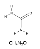
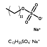
Here we will examine the self-assembly of a ​surfactant, ​sodium dodecyl sulfate (SDS) in the deep eutectic solvent formed from a 1:2 molar ratio mixture of ​choline chloride and ​urea.

Sodium Dodecyl Sulfate	Choline Chloride	Urea

TASK 11: If you haven't already done so, download the SANS data : SwednessSasViewTutorialData.zip​ and unzip the file in a known location on your filesystem. Note where you have placed the data.

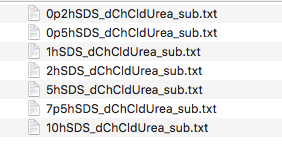
You should now have a folder called "Subtracted" containing a set of files named as follows:

The data are SANS curves collected on SANS2D at ISIS and D22 at ILL for samples of protonated (normal) SDS in 1:2 d9-choline chloride:d4-urea. This sample was chosen to give maximum contrast and minimum background signal from incoherent scattering. There were 7 samples with 0.2 wt%, 0.5 wt%, 1.0 wt%, 2.0 wt%, 5.0 wt%, 7.5 wt% and 10 wt% of SDS in the DES with the filenames corresponding to each sample given below:

Surfactant Concentration (wt%)	Data File
0.2	0p2hSDS_dChCldUrea_sub.txt
0.5	0p5hSDS_dChCldUrea_sub.txt
1.0	1hSDS_dChCldUrea_sub.txt
2.0	2hSDS_dChCldUrea_sub.txt
5.0	5hSDS_dChCldUrea_sub.txt
7.5	7p5hSDS_dChCldUrea_sub.txt
10.0	10hSDS_dChCldUrea_sub.txt

All the data files have been processed to 1D scattering curves with the solvent background subtracted to leave only the coherent scattering signal on absolute scale.

Additionally there is a folder called "Not subtracted" containing the data for task 14.

4.2 Evaluation of the subtracted data

You will now load the background subtracted data into SasView and make a plot in order to visually inspect the scattering curves.

TASK 14: Restart SasView

Before starting this part of the exercise, you should have a clean SasView instance. Quit SasView and restart it.

TASK 15: Click on the "Load Data" button in the Data Explorer

Locate the folder where you placed the data, select all the files in the "subtracted" folder and click "Open" in the dialog.

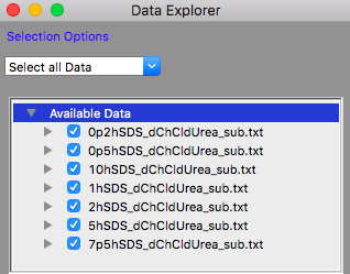
The Available Data section of the Data Explorer should look something like:

TASK 16: Plot the loaded data

Make sure that all the datasets have check marks next to them in the Available Data section of the Data Explorer, as shown above.

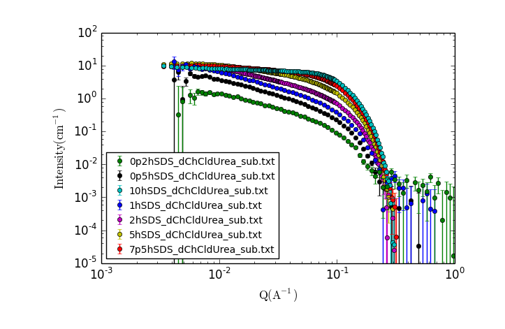
Click the "New Plot" button in the Data Explorer.

A new window should appear with a plot of the data that looks something like:

TASK 17: Examining the Data.

Visually inspect the data, zooming in and making additional plots as needed.

• What trends do you notice?
• What can you say about the possible solution structure from looking at the data?

4.3 Guiner and Kratky Plots

TASK 18: Guiner Analysis

Select the lowest concentration data only in the data explorer by ensuring only 0p2hSDS_dChCldUrea_sub.txt has a check mark next to it and click “Send to" fitting.

• Perform a guinier analysis

TASK 19: Kratky Plot

Select the lowest concentration data only in the data explorer by ensuring only 0p2hSDS_dChCldUrea_sub.txt has a check mark next to it and click “Send to" fitting.

• Make a Kratky plot

What's Next?

You can now move on to the next exercise SLD Calculation and Data Fitting

Resources

• NIST SLD calculator ​https://www.ncnr.nist.gov/resources/activation/
• NIST Scattering Length and Scattering Cross Section Database ​https://www.ncnr.nist.gov/resources/n-lengths/