| Version 37 (modified by ajj, 8 years ago) (diff) |
|---|
Exercise 9 - SANS Data Analysis using SasView
Introduction
This exercise will introduce you to analysing SANS data using geometrical models in SasView. You will first look at how different shapes produce different scattering patterns, and how the model parameters affect the scattering pattern. You will then load some real SANS data and attempt to fit models to the data in SasView.
The exercise is divided into 3 sections:
Before beginning the exercise, you must first ensure that SasView is installed. If you have not done so already, follow these installation instructions.
Tasks you should perform are shown thus:
TASK 0: Install SasView. Installation instructions can be found here: TartuSchoolSasViewInstall
1. Familiarisation with SasView
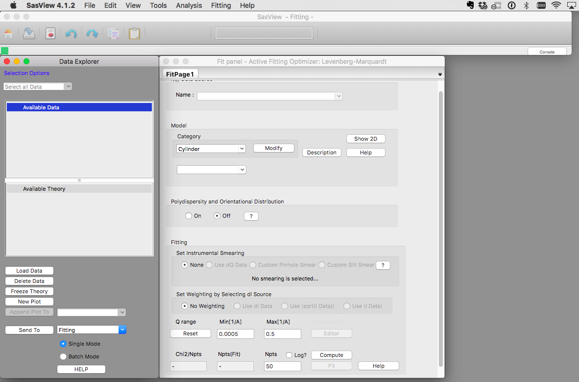
TASK 1: Start SasView. The application should open and look something like the images below.
 | 
|
| SasView 4.1.2 on Mac OS | SasView 4.1.2 on Windows 10 |
The SasView user interface contains 4 main areas:
- The Data Explorer
- This is where data is loaded and can then be plotted or sent to the various types of analysis.
- Models not associated with data (called "Theories" in !Sasview) can be plotted and converted to datasets.
- The Analysis Panel (which defaults to showing Fitting)
- This is where you do the work of analysing data or generating theories
- SasView currently supports four analysis tools:
- Fitting - for theory generation or model fitting to 1D and 2D SANS, SAXS, or SESANS data
- P(r) Inversion - for converting I(Q) to P(r)
- Invariant - for calculating the scattering invariant from a 1D data set
- Correlation Function - for performing a correlation function analysis of a 1D data set
- The plot windows (which appear when something is plotted)
- The menus, toolbar, and status area.
The capabilities of SasView are described in more detail in the application documentation with links to the relevant parts of the documentation available as "Help" buttons in each part of the GUI.
TASK 2: Briefly familiarise yourself with SasView panels, menus and documentation. Try changing to different analysis tools.
2. Exploring geometrical models
In this part of the exercise, you will plot the scattering patterns calculated using different geometrical models and explore the effect that the model parameters have on the scattering.
TASK 3: Restart SasView
Before starting this part of the exercise, you should have a clean SasView instance. Quit SasView and restart it.
2.1 Spheres
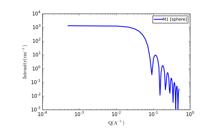
TASK 4: Plot the scattering from a collection of spherical particles
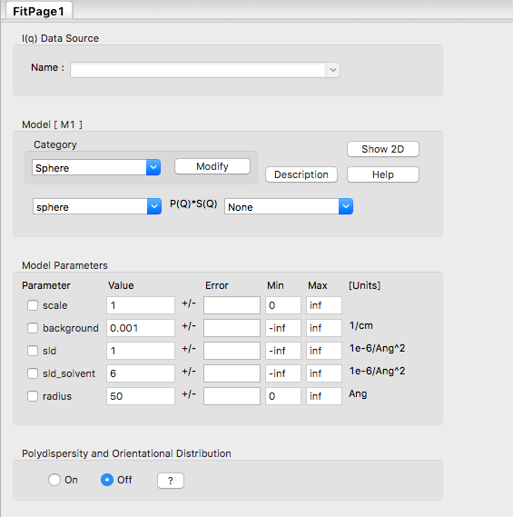
In the Fit Panel, there should be a single tab labelled "Fitpage1". In that tab, choose the model category "Sphere" and the model "sphere".
The fit panel and a plot panel that appears should look like the following:


TASK 5: Change the parameters and note the changes in the scattering pattern.
In the "Fitpage1" tab, scroll down to the bottom and:
- Increase "Npts" to 200
- Check the "Log" box
Next, click "Compute"
This will improve the fidelity of the modelled curve.
Now scroll back up and try adjusting the various model parameters one at a time. Pressing enter after changing a value should recalculate the scattering. If not, use the Compute button.
What effect do the each of the parameters have on the scattering curve?
- scale
- background
- sld and sld_solvent
- radius
2.2 Cylinders
TASK 6: Plot the scattering from a collection of cylindrical particles
From the "Fitting" menu, select "New Fit Page".
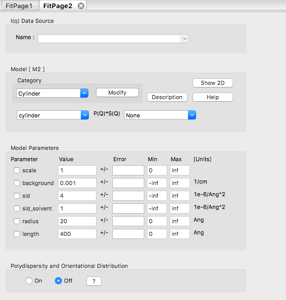
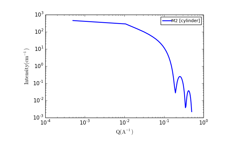
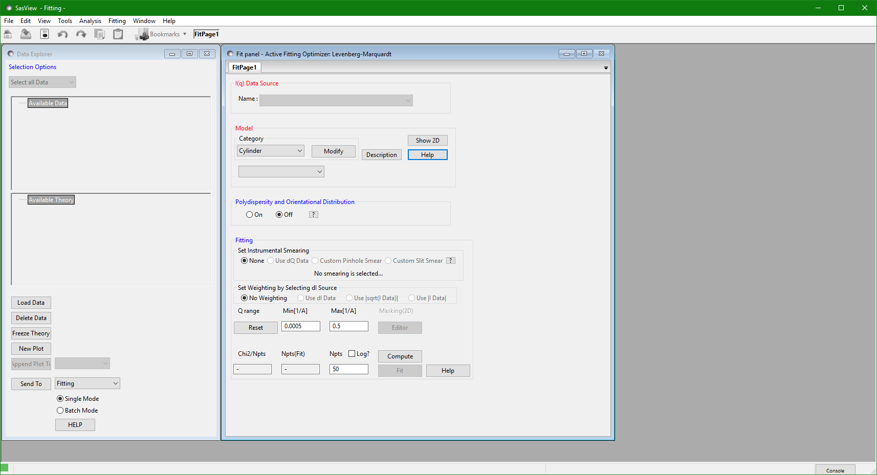
In the Fit panel, a new tab labelled "Fitpage2" should appear. In that tab, choose the model category "Cylinder" and the model "cylinder".
The fit panel and a plot panel that appears should look like the following:


TASK 7: Change the parameters and note the changes in the scattering pattern.
In the "Fitpage2" tab, scroll down to the bottom and:
- Increase "Npts" to 200
- Check the "Log" box
Next, click "Compute"
This will improve the fidelity of the modelled curve.
Now scroll back up and try adjusting the various model parameters one at a time. Pressing enter after changing a value should recalculate the scattering. If not, use the Compute button.
What effect do the each of the parameters have on the scattering curve?
- scale
- background
- sld and sld_solvent
- radius
- length
2.3 Polydispersity
TASK 8: Apply polydispersity to model parameters
Select the "Fitpage1" tab that contains the sphere model.
Find the section labelled "Polydispersity and Orientational Distribution"
Click the "On" radio button and a new section should appear labelled "Distribution of radius".
Enter a value for "PD[ratio]" between 0.0 and 1.0 - this is the polydispersity defined as sigma_r/r.
What effect does varying the polydispersity have on the scattering curve?
Repeat the exercise for the cylinder model in "Fitpage2"
3. Fitting SANS data
This part of the exercise will use real SANS data taken from a study of surfactant self assembly in deep eutectic solvents (DES).
TASK 9: Restart SasView
Before starting this part of the exercise, you should have a clean SasView instance. Quit SasView and restart it.
3.1 Background Information
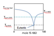
Deep eutectic solvents are a class of ionic liquids formed from a hydrogen bond donor and a halide salt. At a certain mixture ratio, the eutectic mixture, the melting point is significantly depressed to values below room temperature.
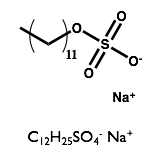
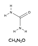
Here we will examine the self-assembly of a surfactant, sodium dodecyl sulfate (SDS) in the deep eutectic solvent formed from a 1:2 molar ratio mixture of choline chloride and urea.
| Sodium Dodecyl Sulfate | Choline Chloride | Urea |
 |  | 
|
TASK 10: Download the SANS data : TartuSasViewTutorialData.zip and unzip the file in a known location on your filesystem. Note where you have placed the data.
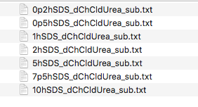
You should now have a folder containing a set of files named as follows:

The data are SANS curves collected on SANS2D at ISIS and D22 at ILL for samples of protonated (normal) SDS in 1:2 d9-choline chloride:d4-urea. This sample was chosen to give maximum contrast and minimum background signal from incoherent scattering. There were 7 samples with 0.2 wt%, 0.5 wt%, 1.0 wt%, 2.0 wt%, 5.0 wt%, 7.5 wt% and 10 wt% of SDS in the DES with the filenames corresponding to each sample given below:
| Surfactant Concentration (wt%) | Data File |
| 0.2 | 0p2hSDS_dChCldUrea_sub.txt |
| 0.5 | 0p5hSDS_dChCldUrea_sub.txt |
| 1.0 | 1hSDS_dChCldUrea_sub.txt |
| 2.0 | 2hSDS_dChCldUrea_sub.txt |
| 5.0 | 5hSDS_dChCldUrea_sub.txt |
| 7.5 | 7p5hSDS_dChCldUrea_sub.txt |
| 10.0 | 10hSDS_dChCldUrea_sub.txt |
All the data files have been processed to 1D scattering curves with the solvent background subtracted to leave only the coherent scattering signal on absolute scale.
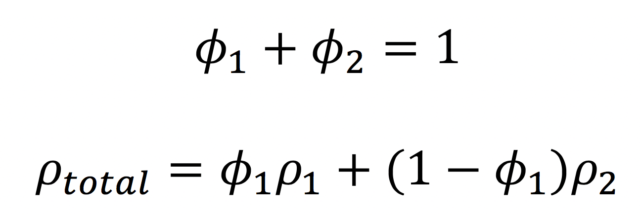
3.2 Calculating Scattering Length Density
The scattering length density is given by

Scattering lengths of relevant elements:
| Element | Scattering Length (fm) |
|---|---|
| C | 6.646 |
| H | -3.739 |
| D | 6.671 |
| N | 9.36 |
| O | 5.803 |
| Cl | 9.577 |
Physical properties of the DES components:
| Component | Chemical Formula | Molecular Volume (Å3) | Density (g/cm3) |
|---|---|---|---|
| d9-Choline Chloride | C5H5D9NOCl | 75.55 | 1.17 |
| d4-Urea | CD4N2O | 210.77 | 1.41 |
TASK 11: Calculate the scattering length density (SLD) of a 1:2 mole ratio mixture of choline chloride and urea.
Use the information in the table above to calculate the SLD. There are multiple ways to do so, including:
- Calculating by hand
- Using a spreadsheet
- Using the SLD calculator built in to SasView (in the Tools menu).
- Using online calculators e.g. https://www.ncnr.nist.gov/resources/activation/
Try multiple ways and see if you get the same answer!
3.3 Loading and Plotting the data
You will now load the data into SasView and make a plot in order to visually inspect the scattering curves.
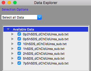
TASK 12: Click on the "Load Data" button in the Data Explorer
Locate the folder where you placed the data, select all the files in that folder and click "Open" in the dialog.
The Available Data section of the Data Explorer should look something like:

TASK 13: Plot the loaded data
Make sure that all the datasets have check marks next to them in the Available Data section of the Data Explorer, as shown above.
Click the "New Plot" button in the Data Explorer.
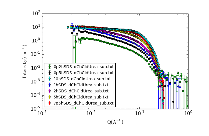
A new window should appear with a plot of the data that looks something like:

TASK 14: Examining the Data.
Visually inspect the data, zooming in and making additional plots as needed.
- What trends do you notice?
- What can you say about the possible solution structure from looking at the data?
3.4 Fitting the data
TASK 15: Fitting the lowest concentration data.
Select the lowest concentration data only in the data explorer by ensuring only 0p2hSDS_dChCldUrea_sub.txt has a check mark next to it and click “Send to" fitting.
- Select the model for the structure you predicted for this dataset.
- How does it compare to the data?
- Fill in parameters you know and adjust the others to see how close you get to the data.
- Select parameters to fit and run the fit by clicking "Fit" at the bottom of the fitting panel.
- Do you get a good fit?
- Are the parameters you get physically reasonable?
TASK 16: Fitting the other data, starting with the 7.5 wt% data set.
Repeat for other concentrations
- Does the same model fit all data?
- What is consistent between datasets? What is different?
Resources
- The original paper and supplementary information
- NIST SLD calculator https://www.ncnr.nist.gov/resources/activation/
- NIST Scattering Length and Scattering Cross Section Database https://www.ncnr.nist.gov/resources/n-lengths/
Attachments (18)
-
tartu_choline.png
(10.8 KB) -
added by ajj 8 years ago.
Structure of choline chloride
-
tartu_sds.png
(12.5 KB) -
added by ajj 8 years ago.
Structure of SDS
-
tartu_urea.png
(10.9 KB) -
added by ajj 8 years ago.
Structure of Urea
-
tartu_des.png
(16.7 KB) -
added by ajj 8 years ago.
A deep eutectic
-
TartuSasViewTutorialData.zip
(29.7 KB) -
added by ajj 8 years ago.
Tartu SasView? Tutorial Data
-
MicelleStructureinDeepEutecticSolvents.pdf
(3.5 MB) -
added by ajj 8 years ago.
PCCP Paper on Surfactants in DES
- tartu_loaddata.png (29.5 KB) - added by ajj 8 years ago.
- tartu_dataplot.png (69.7 KB) - added by ajj 8 years ago.
- tartu_sld.png (11.0 KB) - added by ajj 8 years ago.
- tartu_datafileslist.png (33.8 KB) - added by ajj 8 years ago.
- tartu_fitpage1_1.png (60.7 KB) - added by ajj 8 years ago.
- tartu_fitpage2_1.png (64.2 KB) - added by ajj 8 years ago.
- tartu_cylinder.png (23.1 KB) - added by ajj 8 years ago.
- tartu_sphere.png (24.2 KB) - added by ajj 8 years ago.
- tartu_sasviewmac.png (158.7 KB) - added by ajj 8 years ago.
- tartu_sasviewwin.png (55.3 KB) - added by ajj 8 years ago.
- MicelleStructureinDeepEutecticSolventsSupplementaryInformation.pdf (3.9 MB) - added by ajj 8 years ago.
- kemm37_volumefraction_sld.png (122.6 KB) - added by ajj 7 years ago.