| Version 3 (modified by ajj, 7 years ago) (diff) |
|---|
Exercise 9 - SANS Data Analysis using SasView
Introduction
This exercise will introduce you to analysing SANS data using geometrical models in SasView. You will first look at how different shapes produce different scattering patterns, and how the model parameters affect the scattering pattern. You will then load some real SANS data and attempt to fit models to the data in SasView.
The exercise is divided into 3 sections:
Before beginning the exercise, you must first ensure that SasView is installed. If you have not done so already, follow these installation instructions.
1. Familiarisation with SasView
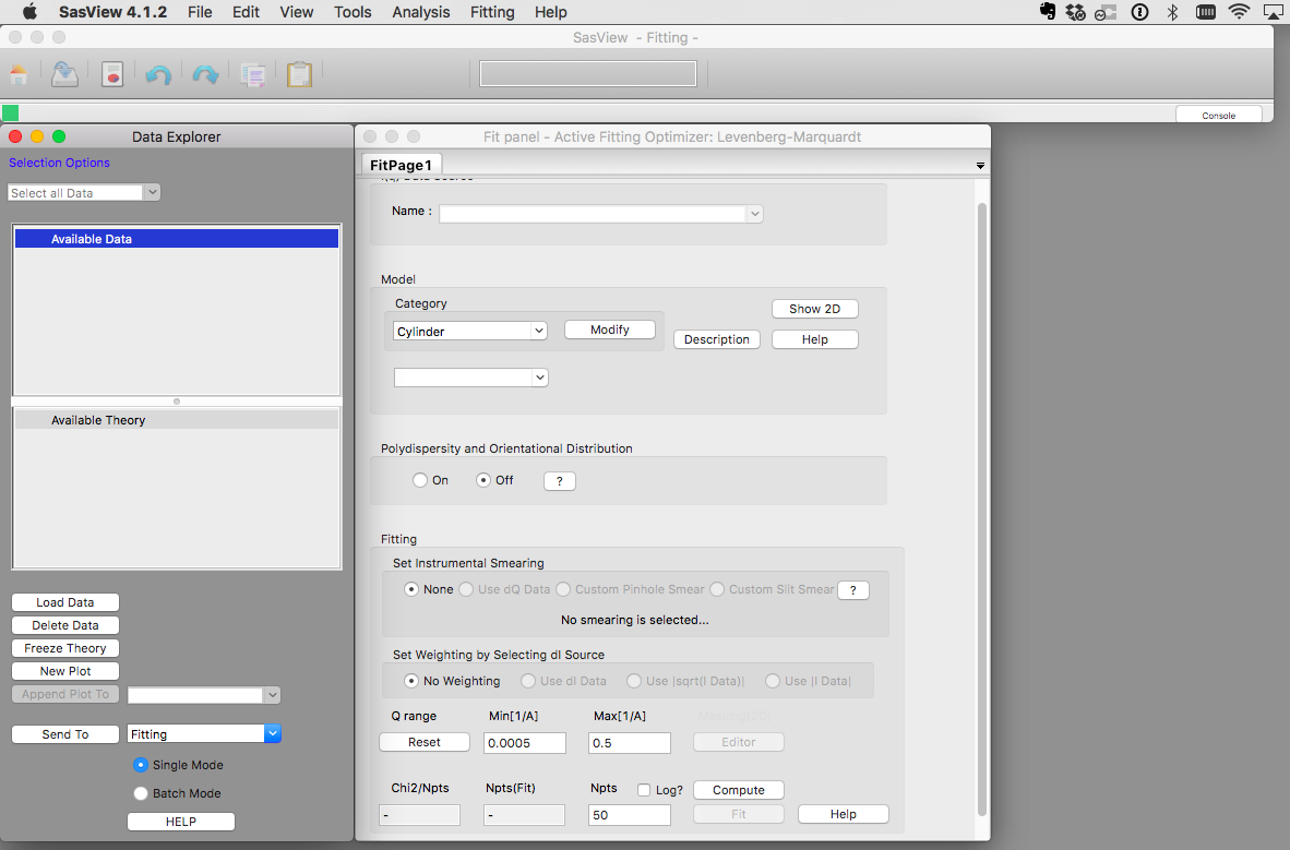
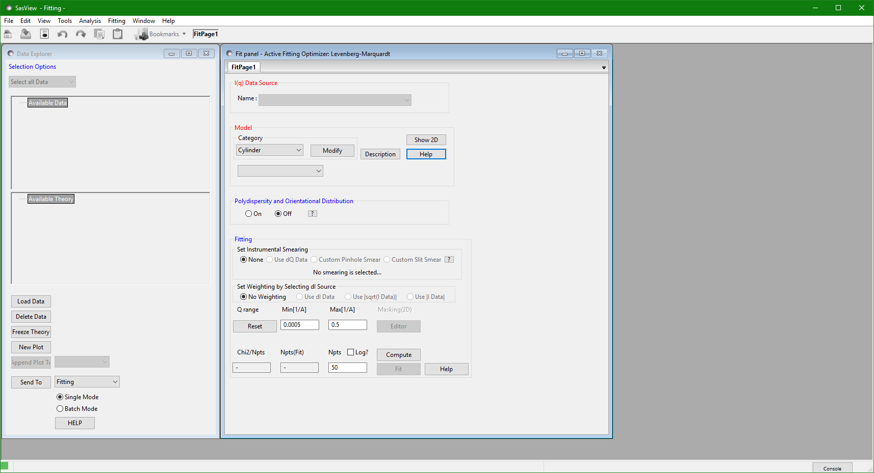
Start SasView. The application should open and look something like the images below.
The SasView user interface contains 4 main areas:
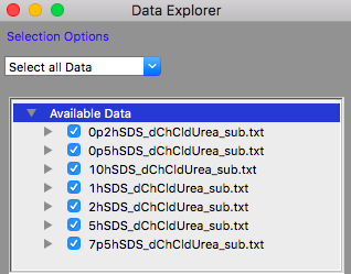
- The Data Explorer
- This is where data is loaded and can then be plotted or sent to the various types of analysis.
- Models not associated with data (called "Theories" in !Sasview) can be plotted and converted to datasets.
- The Analysis Panel (which defaults to showing Fitting)
- This is where you do the work of analysing data or generating theories
- SasView currently supports four analysis tools:
- Fitting - for theory generation or model fitting to 1D and 2D SANS, SAXS, or SESANS data
- P(r) Inversion - for converting I(Q) to P(r)
- Invariant - for calculating the scattering invariant from a 1D data set
- Correlation Function - for performing a correlation function analysis of a 1D data set
- The plot windows (which appear when something is plotted)
- The menus, toolbar, and status area.
The capabilities of SasView are described in more detail in the [ application documentation] with links to the documentation available as "Help" buttons in each part of the GUI.
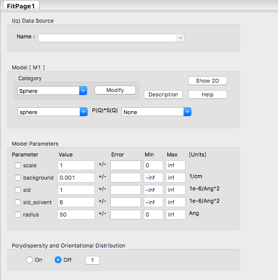
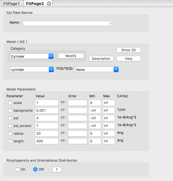
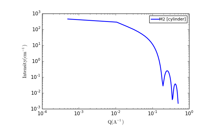
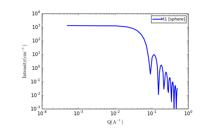
2. Exploring geometrical models
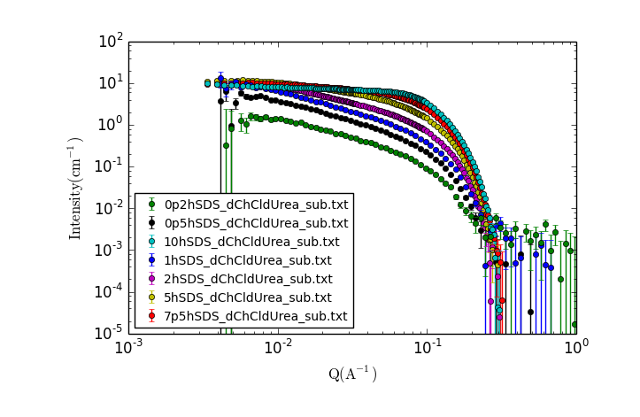
3. Fitting SANS data
Attachments (18)
-
tartu_choline.png
(10.8 KB) -
added by ajj 7 years ago.
Structure of choline chloride
-
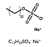
tartu_sds.png
(12.5 KB) -
added by ajj 7 years ago.
Structure of SDS
-
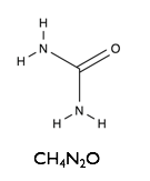
tartu_urea.png
(10.9 KB) -
added by ajj 7 years ago.
Structure of Urea
-
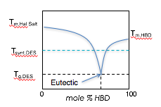
tartu_des.png
(16.7 KB) -
added by ajj 7 years ago.
A deep eutectic
-
TartuSasViewTutorialData.zip
(29.7 KB) -
added by ajj 7 years ago.
Tartu SasView? Tutorial Data
-
MicelleStructureinDeepEutecticSolvents.pdf
(3.5 MB) -
added by ajj 7 years ago.
PCCP Paper on Surfactants in DES
- tartu_loaddata.png (29.5 KB) - added by ajj 7 years ago.
- tartu_dataplot.png (69.7 KB) - added by ajj 7 years ago.
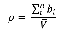
- tartu_sld.png (11.0 KB) - added by ajj 7 years ago.
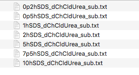
- tartu_datafileslist.png (33.8 KB) - added by ajj 7 years ago.
- tartu_fitpage1_1.png (60.7 KB) - added by ajj 7 years ago.
- tartu_fitpage2_1.png (64.2 KB) - added by ajj 7 years ago.
- tartu_cylinder.png (23.1 KB) - added by ajj 7 years ago.
- tartu_sphere.png (24.2 KB) - added by ajj 7 years ago.
- tartu_sasviewmac.png (158.7 KB) - added by ajj 7 years ago.
- tartu_sasviewwin.png (55.3 KB) - added by ajj 7 years ago.
- MicelleStructureinDeepEutecticSolventsSupplementaryInformation.pdf (3.9 MB) - added by ajj 7 years ago.
- kemm37_volumefraction_sld.png (122.6 KB) - added by ajj 6 years ago.