KEMM37 Lab 1B - SANS Data Analysis using SasView

Table of Contents
3. Fitting SANS data
3.1 Background Information
3.2 Calculating Scattering Length Density
3.3 Loading and Plotting the data
3.4 Fitting the data
Resources

3. Fitting SANS data

This part of the exercise will use real SANS data taken from a study of surfactant self assembly in deep eutectic solvents (DES).

TASK 10: Restart SasView

Before starting this part of the exercise, you should have a clean SasView instance. Quit SasView and restart it.

3.1 Background Information

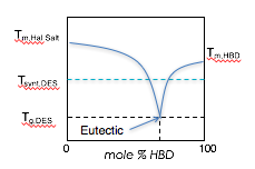
Deep eutectic solvents are a class of ionic liquids formed from a hydrogen bond donor and a halide salt. At a certain mixture ratio, the eutectic mixture, the melting point is significantly depressed to values below room temperature.

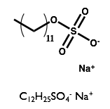
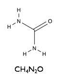
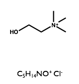
Here we will examine the self-assembly of a ​surfactant, ​sodium dodecyl sulfate (SDS) in the deep eutectic solvent formed from a 1:2 molar ratio mixture of ​choline chloride and ​urea.

Sodium Dodecyl Sulfate	Choline Chloride	Urea

TASK 11: Download the SANS data : KEMM37SasViewTutorialData.zip​ and unzip the file in a known location on your filesystem. Note where you have placed the data.

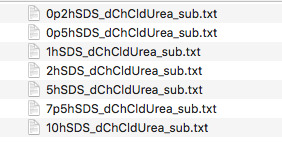
You should now have a folder called "Subtracted" containing a set of files named as follows:

The data are SANS curves collected on SANS2D at ISIS and D22 at ILL for samples of protonated (normal) SDS in 1:2 d9-choline chloride:d4-urea. This sample was chosen to give maximum contrast and minimum background signal from incoherent scattering. There were 7 samples with 0.2 wt%, 0.5 wt%, 1.0 wt%, 2.0 wt%, 5.0 wt%, 7.5 wt% and 10 wt% of SDS in the DES with the filenames corresponding to each sample given below:

Surfactant Concentration (wt%)	Data File
0.2	0p2hSDS_dChCldUrea_sub.txt
0.5	0p5hSDS_dChCldUrea_sub.txt
1.0	1hSDS_dChCldUrea_sub.txt
2.0	2hSDS_dChCldUrea_sub.txt
5.0	5hSDS_dChCldUrea_sub.txt
7.5	7p5hSDS_dChCldUrea_sub.txt
10.0	10hSDS_dChCldUrea_sub.txt

All the data files have been processed to 1D scattering curves with the solvent background subtracted to leave only the coherent scattering signal on absolute scale.

Additionally there is a folder called "Not subtracted" containing the data for task 14.

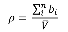
3.2 Calculating Scattering Length Density

The scattering length density is given by

Scattering lengths of relevant elements:

Element	Scattering Length (fm)
C	6.646
H	-3.739
D	6.671
N	9.36
O	5.803
Cl	9.577

Physical properties of the DES components:

Component	Chemical Formula	Molecular Volume (Å3)	Density (g/cm3)
d9-Choline Chloride	C5H5D9NOCl	210.77	1.17
d4-Urea	CD4N2O	75.55	1.41

TASK 12: Calculate the scattering length density (SLD) of a 1:2 mole ratio mixture of choline chloride and urea.

Use the information in the table above to calculate the SLD. There are multiple ways to do so, including:

• Calculating by hand
• Using a spreadsheet
• Using the SLD calculator built in to SasView (in the Tools menu).
• Using online calculators e.g. ​https://www.ncnr.nist.gov/resources/activation/

Try calculating by hand and one or more of the other ways and see if you get the same answer!

3.5 Loading data and Subtracting a Solvent Background

You will now load in the original reduced data for the 0.5 wt% concentration of SDS and subtract the solvent background from it.

TASK 13: Click on the "Load Data" button in the Data Explorer

Locate the folder where you placed the data, select all the files in the "Not subtracted" folder and click "Open" in the dialog.

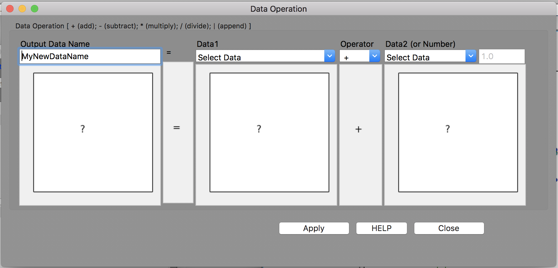
TASK 14: Subtract the solvent background using the "Data Operation" Tool

From the "Tools" menu, select "Data Operation".

You should have a window that looks something like this:

Give your output data set a name of your choosing in the "Output Data Name" box

In the "Data 1" drop down, select the sample data set "0p5hSDS_dChCldUrea.txt".

In the "Operator" drop down, choose "-" (minus)

In the "Data 2" drop down, select the solvent data set "dChCldUrea.txt".

Click "Apply", then "Close"

In the data explorer, there should now be a data set with the name you chose above.

Make a plot of the original data sets and your subtracted one to compare them and check you did the subtraction correctly. Make sure that there are check marks next to "0p5hSDS_dChCldUrea.txt", "dChCldUrea.txt", and the dataset with the name you chose. Click on "New Plot" at the bottom of the Data Explorer.

Does the result look reasonable? What effects have subtracting the solvent scattering from the sample scattering had on the scattering curve? What are possible sources of the background signal that you are removing?

3.4 Loading and Plotting the subtracted data

You will now load the background subtracted data into SasView and make a plot in order to visually inspect the scattering curves.

TASK 15: Restart SasView

Before starting this part of the exercise, you should have a clean SasView instance. Quit SasView and restart it.

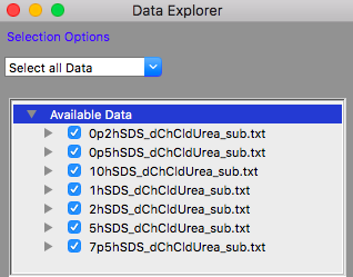
TASK 16: Click on the "Load Data" button in the Data Explorer

Locate the folder where you placed the data, select all the files in the "subtracted" folder and click "Open" in the dialog.

The Available Data section of the Data Explorer should look something like:

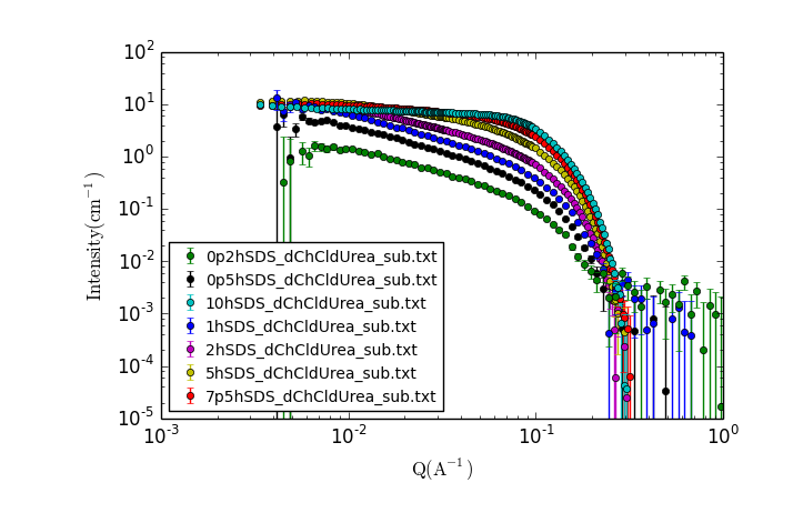
TASK 17: Plot the loaded data

Make sure that all the datasets have check marks next to them in the Available Data section of the Data Explorer, as shown above.

Click the "New Plot" button in the Data Explorer.

A new window should appear with a plot of the data that looks something like:

TASK 18: Examining the Data.

Visually inspect the data, zooming in and making additional plots as needed.

• What trends do you notice?
• What can you say about the possible solution structure from looking at the data?

3.5 Fitting the data

TASK 19: Fitting the lowest concentration data.

Select the lowest concentration data only in the data explorer by ensuring only 0p2hSDS_dChCldUrea_sub.txt has a check mark next to it and click “Send to" fitting.

• Select the model for the structure you predicted for this dataset.
  • How does it compare to the data?
• Fill in parameters you know and adjust the others to see how close you get to the data.
• Select parameters to fit and run the fit by clicking "Fit" at the bottom of the fitting panel.
  • Do you get a good fit?
  • Are the parameters you get physically reasonable?

TASK 20: Fitting the other data, starting with the 7.5 wt% data set.

Repeat for other concentrations

• Does the same model fit all data?
• What is consistent between datasets? What is different?

TASK 21: Summarising the results

Having fitted all the data sets you can now summarise the results and comment on the trends you observe.

What's Next?

You can now move on to finishing your lab report - details are here : KEMM37 Lab 1 Report

Resources

• NIST SLD calculator ​https://www.ncnr.nist.gov/resources/activation/
• NIST Scattering Length and Scattering Cross Section Database ​https://www.ncnr.nist.gov/resources/n-lengths/