| Version 4 (modified by ajj, 7 years ago) (diff) |
|---|
Exercise 9 - SANS Data Analysis using SasView
| Table of Contents |
|---|
| Introduction |
| 1. Familiarisation with SasView |
| 2. Exploring geometrical models |
| 2.1 Spheres |
| 2.2 Cylinders |
| 2.3 Polydispersity |
| 2.4 Resolution |
Introduction
This exercise will introduce you to analysing SANS data using geometrical models in SasView. You will first look at how different shapes produce different scattering patterns, and how the model parameters affect the scattering pattern. You will then load some real SANS data and attempt to fit models to the data in SasView.
The exercise is divided into 3 sections:
Before beginning the exercise, you must first ensure that SasView is installed. If you have not done so already, follow these installation instructions?.
Tasks you should perform are shown thus:
TASK 0: Install SasView. Installation instructions can be found here: KEMM37/InstallSasview?
1. Familiarisation with SasView
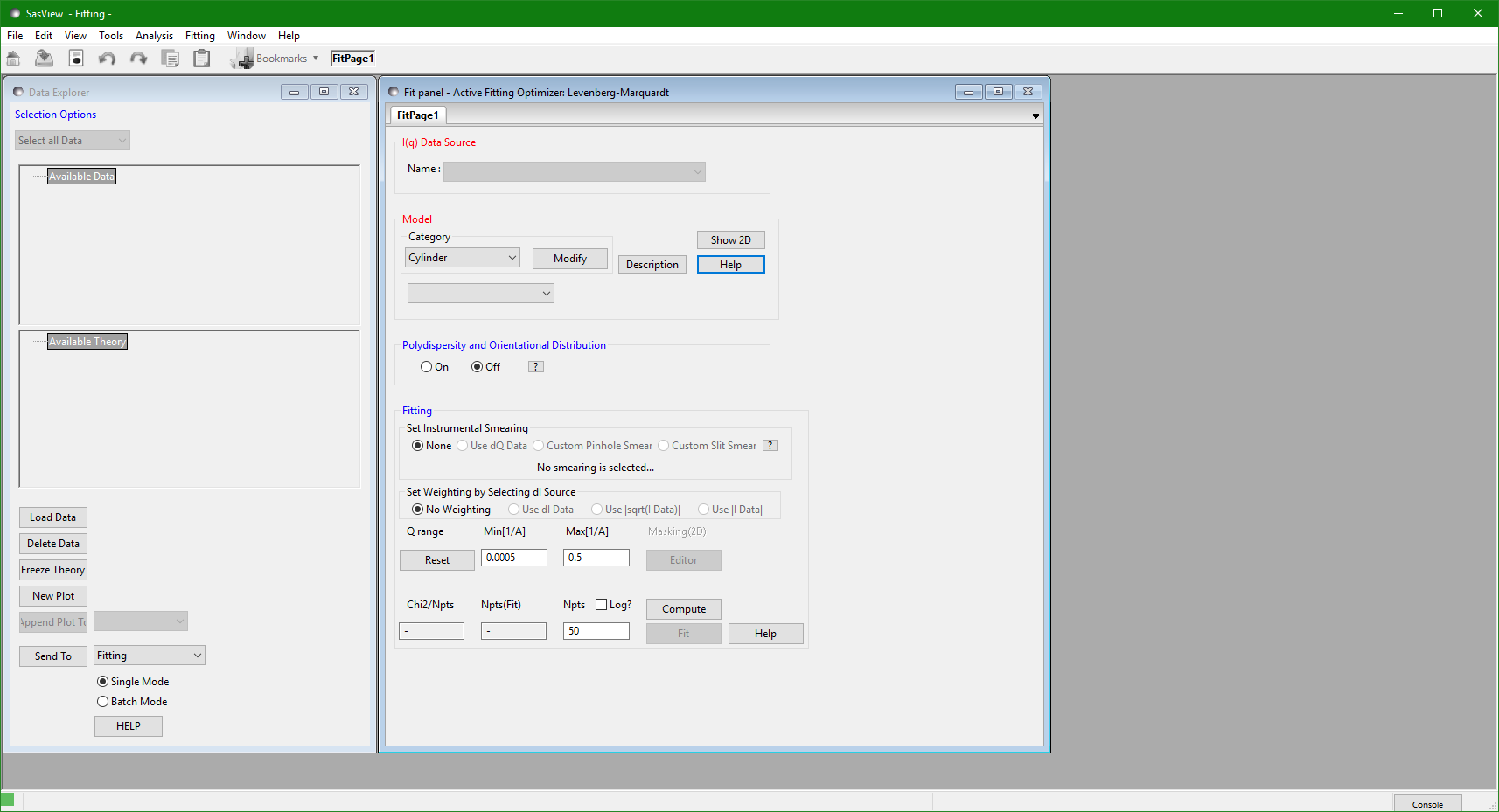
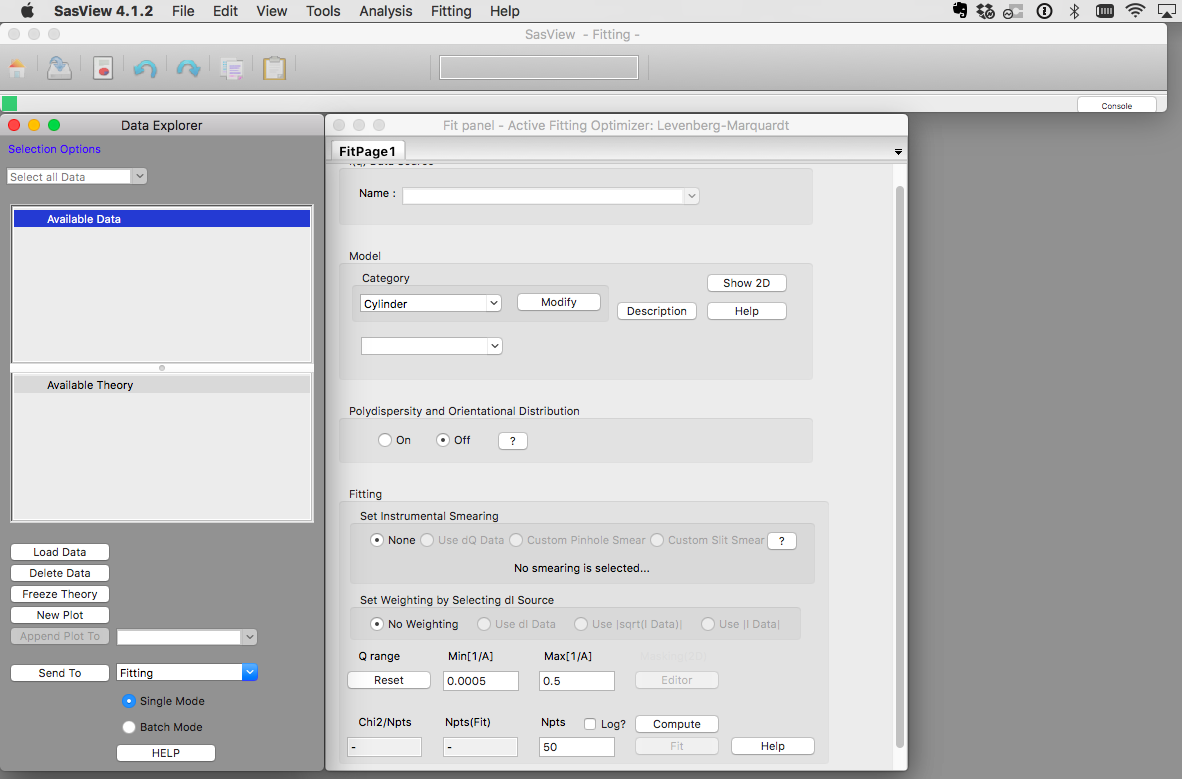
TASK 1: Start SasView. The application should open and look something like the images below.
 | 
|
| SasView 4.1.2 on Mac OS | SasView 4.1.2 on Windows 10 |
The SasView user interface contains 4 main areas:
- The Data Explorer
- This is where data is loaded and can then be plotted or sent to the various types of analysis.
- Models not associated with data (called "Theories" in !Sasview) can be plotted and converted to datasets.
- The Analysis Panel (which defaults to showing Fitting)
- This is where you do the work of analysing data or generating theories
- SasView currently supports four analysis tools:
- Fitting - for theory generation or model fitting to 1D and 2D SANS, SAXS, or SESANS data
- P(r) Inversion - for converting I(Q) to P(r)
- Invariant - for calculating the scattering invariant from a 1D data set
- Correlation Function - for performing a correlation function analysis of a 1D data set
- The plot windows (which appear when something is plotted)
- The menus, toolbar, and status area.
The capabilities of SasView are described in more detail in the application documentation with links to the relevant parts of the documentation available as "Help" buttons in each part of the GUI.
TASK 2: Briefly familiarise yourself with SasView panels, menus and documentation. Try changing to different analysis tools.
2. Exploring geometrical models
In this part of the exercise, you will plot the scattering patterns calculated using different geometrical models and explore the effect that the model parameters have on the scattering.
TASK 3: Restart SasView
Before starting this part of the exercise, you should have a clean SasView instance. Quit SasView and restart it.
2.1 Spheres
TASK 4: Plot the scattering from a collection of spherical particles
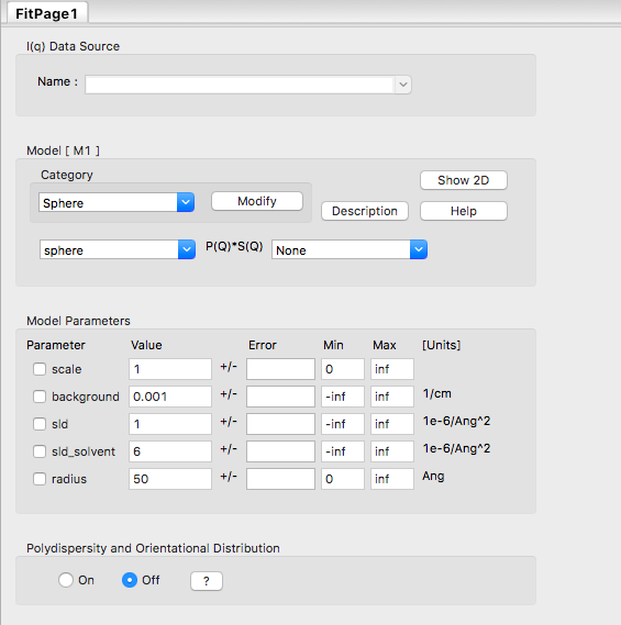
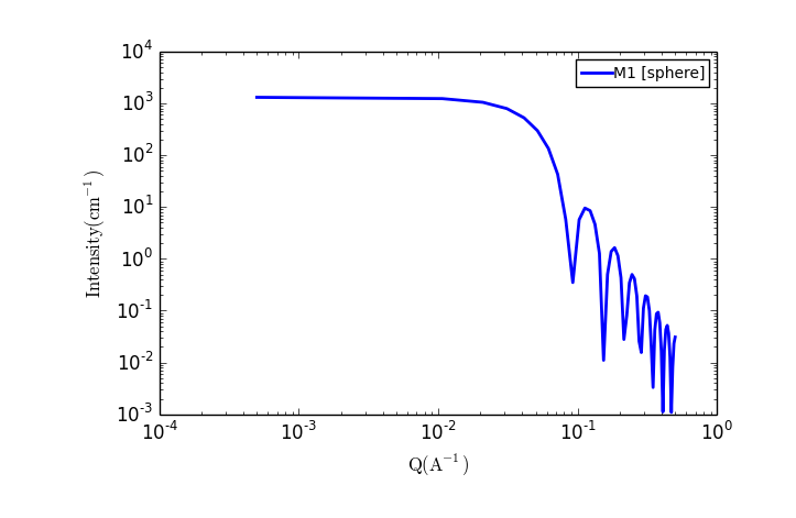
In the Fit Panel, there should be a single tab labelled "Fitpage1". In that tab, choose the model category "Sphere" and the model "sphere".
The fit panel and a plot panel that appears should look like the following:


TASK 5: Change the parameters and note the changes in the scattering pattern.
In the "Fitpage1" tab, scroll down to the bottom and:
- Increase "Npts" to 200
- Check the "Log" box
Next, click "Compute"
This will improve the fidelity of the modelled curve.
Now scroll back up and try adjusting the various model parameters one at a time. Pressing enter after changing a value should recalculate the scattering. If not, use the Compute button.
What effect do the each of the parameters have on the scattering curve?
- scale
- background
- sld and sld_solvent
- radius
2.2 Cylinders
TASK 6: Plot the scattering from a collection of cylindrical particles
From the "Fitting" menu, select "New Fit Page".
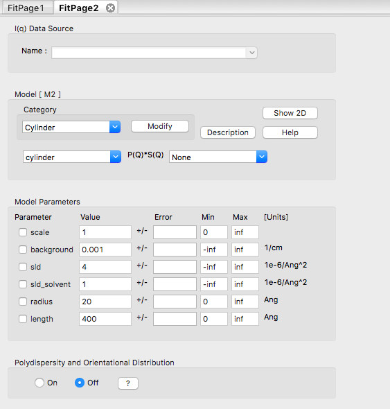
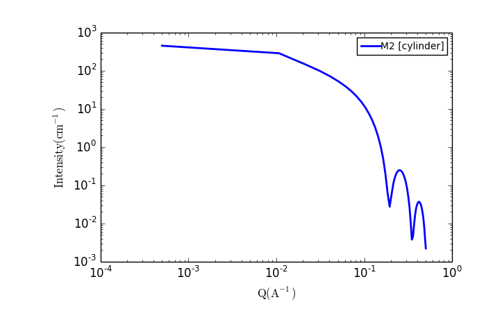
In the Fit panel, a new tab labelled "Fitpage2" should appear. In that tab, choose the model category "Cylinder" and the model "cylinder".
The fit panel and a plot panel that appears should look like the following:


TASK 7: Change the parameters and note the changes in the scattering pattern.
In the "Fitpage2" tab, scroll down to the bottom and:
- Increase "Npts" to 200
- Check the "Log" box
Next, click "Compute"
This will improve the fidelity of the modelled curve.
Now scroll back up and try adjusting the various model parameters one at a time. Pressing enter after changing a value should recalculate the scattering. If not, use the Compute button.
What effect do the each of the parameters have on the scattering curve?
- scale
- background
- sld and sld_solvent
- radius
- length
2.3 Polydispersity
TASK 8: Apply polydispersity to model parameters
Select the "Fitpage1" tab that contains the sphere model.
Find the section labelled "Polydispersity and Orientational Distribution"
Click the "On" radio button and a new section should appear labelled "Distribution of radius".
Enter a value for "PD[ratio]" between 0.0 and 1.0 - this is the polydispersity defined as sigma_r/r.
What effect does varying the polydispersity have on the scattering curve?
Repeat the exercise for the cylinder model in "Fitpage2"
2.4 Resolution
TASK 9: Apply resolution functions to your model
What's Next?
You can now move on to the second lab session looking at fitting of data : Lab 1B Data Fitting
Attachments (6)
- kemm37_sasviewwin.png (55.3 KB) - added by ajj 7 years ago.
- kemm37_sasviewmac.png (158.7 KB) - added by ajj 7 years ago.
- kemm37_fitpage2_1.png (64.2 KB) - added by ajj 7 years ago.
- kemm37_cylinder.png (23.1 KB) - added by ajj 7 years ago.
- kemm37_fitpage1_1.png (60.7 KB) - added by ajj 7 years ago.
- kemm37_sphere.png (24.2 KB) - added by ajj 7 years ago.
Download all attachments as: .zip