Opened 7 years ago
Last modified 6 years ago
#805 new defect
improve accuracy of fcc/bcc/sc
| Reported by: | pkienzle | Owned by: | |
|---|---|---|---|
| Priority: | major | Milestone: | SasView 4.3.0 |
| Component: | SasView | Keywords: | |
| Cc: | Work Package: | SasView Bug Fixing |
Description
fcc/bcc/sc paracrystal models use the following expression:
    exp_qd = mp.exp(-qd**2*a/2)
    return (1 - exp_qd**2) / (1 - 2*exp_qd*mp.cos(qd*b) + exp_qd**2)
this can behave poorly for low q, even though the limit exists:
    lim x->0 [(1 - exp(-a x^2)) / (1 - 2*exp(-a x^2/2) cos(b x) + exp(-a x^2)]

    => a/b^2
Maybe replace this with a Taylor expansion at low q so that the model can run in single precision.
Note that there are alternate forms of this expression:
    sinh(ax^2) / (cosh(ax^2) - cos(bx))
    tanh(ax^2) / (1 - cos(bx)/cosh(ax^2)
Attachments (4)
Change History (12)
comment:1 Changed 7 years ago by pkienzle
Changed 7 years ago by pkienzle
Changed 7 years ago by pkienzle
Changed 7 years ago by pkienzle
comment:2 Changed 7 years ago by pkienzle
- Milestone changed from SasView Next Release +1 to SasView 4.2.0
- Priority changed from minor to major
- Type changed from enhancement to defect
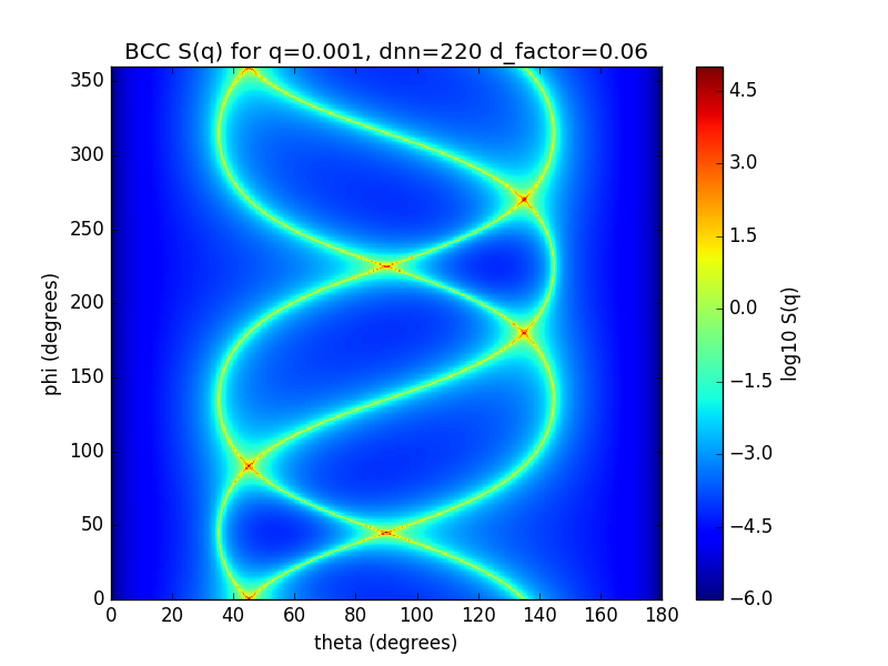
The current 1D calculations for BCC paracrystal are very wrong at low q, orders
of magnitude wrong. The integration fails to capture a very narrow,
very steep ridge.
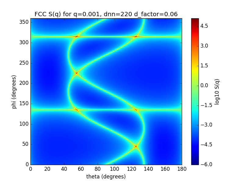
The attached plots show the S(q, theta, phi) values for q=0.001 over the entire 4 pi surface. Note particularly that this is a log scale image spanning many orders of magnitude.
Experimenting with different integration routines, scipy.dblquad can get an accurate value of this integral using 1M evals. simpsons/trapezoid/romberg on a uniform grid require 16M. Adaptive romberg didn't complete in the time that I gave it. The 150x150 gaussian quadrature we are currently using is not adequate. We may need a specialized integrator for low q which can identify and integrate the ridges properly.
Use sasmodels/explore/bccpy.py in the ticket-776-orientation branch to explore integration options and plot the image.
Given the 8-fold symmetry of the cubic system I was expecting to see eight-fold symmetry in the phi-theta map. Any idea why this would not be the case for fcc/bcc? Are we sure the calculation of S(q) is correct for fcc/bcc?


Changed 7 years ago by pkienzle
comment:3 Changed 7 years ago by pkienzle
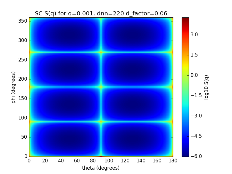
Difference between 150 points and 4000 points in integration of simple cubic model:

comment:4 Changed 7 years ago by pkienzle
(1) Re: valid q range
The integration issue is primarily with q values below the first peak (2 pi/dnn for simple cubic, 2 root 2 pi/dnn for fcc and bcc). The function is okay by the second peak, or sooner if the distortion factor is large. Lowering the lattice distortion exacerbates the problem by making the peaks narrower; this will lead to artificial peak splitting as d_factor goes to zero.
(2) Re: nastiness of the integrand
The images above plot I(q,theta,phi) for the set of theta/phi used when integrating at q=0.001. This shows the narrow ridges traced out by the function that the integration function must deal with.
Some options:
- Is a change of variables which will flatten the peaks? This would be equivalent to adaptive integration, but specialized for this particular function.
- Choose of the number of integration points depend on q, dnn and d_factor. Since we are usually evaluating neighbouring q values in the 1-D case, all threads in a warp should be taking the same branch so the performance hit won't be too nasty.
- Enumerate the contribution from each specific hkl point at low q. We know where they are and how big they are, so we don't need to rely on numerical integration to happen upon them. See below for details.
(3) Re: cryptic doc comment about the validity of the 2D transform
The paper doesn't indicate that any particular approximations have been made in the derivation. Eq 7 is a simple orientational average of eq 6. Section B begins with the statement:
The lattice factor Z(q) for the sc lattice can be calculated by the method of Yarusso et al., Their method is to calculate the diffraction pattern from the assembly of randomly oriented paracrystals by taking a rotational average of one infinitely large paracrystal.
So the finite size effects on the lattice are not taken into account when scattering off less than infinite ordered particle agglomerations, which I'm guessing leads to narrower than expected peak widths. This seems like it would affect the 1D as much as the 2D.
I don't see a reason to keep the comment in the docs.
(4) Re: 8-fold symmetry
I expect the cubic system to show 8-fold symmetry in the phi-theta plot over all possible orientations for a single q because the 8 corners should be indistinguishable as far as the incident neutron is concerned. That is, phi in [0,pi/2] should match phi in [pi/2,pi], [pi, 3pi/2] and [3pi/2, 2pi]. Similarly, I expect theta in [0, pi/2] to match theta in [pi, pi/2].
Note: running explore/bccpy.py with higher d_factor is interesting. It distorts some parts of the sphere differently from other parts.
(5) Re: test values and choice of coordinate systems in the 2D transform
Jae He says the following in his code:
Angles here are respect to detector coordinate instead of against q coordinate
Since I'm already rotating from detector to q before calling this code, I think we need to go back to the original transform from b to a in the paper. Unfortunately, since this is a cubic system we can't just look at the shape along a, b and c axes to make sure we have the correct interpretation of the angles, and actually have to think about where the spots should appear for a given theta, phi.
(6) Re: 1D peak positions as a function of dnn
The parameter to the model is labelled as nearest neighbour distance, but I believe it is lattice spacing.
In units of lattice spacing, a, the q positions of the peaks are well determined by:
q = 2*pi/a * sqrt(h^2 + k^2 + l^2)
where SC allows all integer hkl, BCC requires h+k+l even and FCC require hkl all even or hkl all odd. Also need peak multiplicity, since [100] = [-100] = [010] = [0-10] = [001] = [00-1], etc.
I checked that this is indeed the case for dnn=20 and d_factor=0.06 for sc, bcc and fcc.
We should rename dnn to length_a as in the parallelepiped model, and rename d_factor to lattice_distortion. Lattice distortion is actually Delta a / a, but distortion_proportion is too much of a mouthful.
Here is a table of multiplicities for low q
| HKL | N=h2+k2+l2 | Multiplicity | SC- | BCC | FCC |
|---|---|---|---|---|---|
| 100 | 1 | 6 | SC | ||
| 110 | 2 | 12 | SC | BCC | |
| 111 | 3 | 8 | SC | FCC | |
| 200 | 4 | 6 | SC | BCC | FCC |
| 210 | 5 | 24 | SC | ||
| 211 | 6 | 24 | SC | BCC | |
| —- | 7 | — | |||
| 220 | 8 | 12 | SC | BCC | FCC |
| 221,300 | 9 | 24+6 | SC | ||
| 310 | 10 | 24 | SC | BCC | |
| 311 | 11 | 24 | SC | FCC | |
| 222 | 12 | 8 | SC | BCC | FCC |
| 320 | 13 | 24 | SC | ||
| 321 | 14 | 48 | SC | BCC | |
| —- | 15 | — | |||
| 400 | 16 | 6 | SC | BCC | FCC |
From https://www-thphys.physics.ox.ac.uk/people/SteveSimon/condmat2012/SlidesfromLecture14.pdf
Powder diffraction chapter indicates that total integrated peak intensity also depends on angle according to the Lorentz-polarization factor LP = (1 + cos2 2
comment:5 Changed 7 years ago by richardh
This all begs the question as to whether sasview should be attempting crystallography, fun as it is, or sticking to reasonably well behaved functions. I can see a good case for having the 1d versions of paracrystals, but I'm not so sure about 2d.
comment:6 Changed 7 years ago by richardh
Further note: The paracrystal models are actually a product of an S(Q) for the crystal with a form factor for the particles P(Q). P(Q) is currently assumed sphere, but alas when the sphere is polydisperse the lengthy S(Q) calculation will I think be being needlessly repeated during the polydispersity integration.
Strictly the P(Q) should be removed and the three paracrystal models be set up as S(Q)'s, which can then be combined with P(Q) for spherically averaged particles of any shape. (Would the maths still be correct for oriented particle 2D P(Q), eg. rods all pointing one way ? I suspect yes, though note that the rods would have to be "short" as the S(Q) lattice is cubic.)
comment:7 Changed 6 years ago by butler
- Milestone changed from SasView 4.2.0 to SasView 4.3.0
comment:8 Changed 6 years ago by smk78
Also see #1156
Checking with mpmath, the third form is closer for single precision, though still not particularly good:
import mpmath as mp

def v1(qd,a,b):
    exp_qd = mp.exp(qd**2*a/2)
    sinh_qd = exp_qd/2 - 1/(exp_qd*2)
    cosh_qd = exp_qd/2 + 1/(exp_qd*2)
    return sinh_qd/(cosh_qd - mp.cos(qd*b))

def v2(qd,a,b):
    arg = qd**2*a/2
    tanh_qd = mp.tanh(arg)
    cosh_qd = mp.cosh(arg)
    return tanh_qd/(1 - mp.cos(qd*b)/cosh_qd)

>>> with mp.workdps(50): qd,a,b=1/mp.mpf(10000),1,1; print(v1(qd,a,b), v2(qd,a,b))
0.99999999833333333999999998419312173141534384383611 0.99999999833333333999999998419312173141534364465429

>>> with mp.workdps(15): qd,a,b=1/mp.mpf(10000),1,1; print(v1(qd,a,b), v2(qd,a,b))
1.0 1.00000000607747

>>> with mp.workdps(7): qd,a,b=1/mp.mpf(10000),1,1; print(v1(qd,a,b), v2(qd,a,b))
0.0 0.6710886
The original form is usually better but sometimes worse:
def v3(qd,a,b):
    exp_qd = mp.exp(-qd**2*a/2)
    exp_qd_sq = mp.exp(-qd**2*a)
    return (1 - exp_qd_sq) / (1 - 2*exp_qd*mp.cos(qd*b) + exp_qd_sq)
None of them are good enough for single precision yet.