Smear Computation

• Slit Smear
• Pinhole Smear
• 2D Smear

Slit Smear

The sit smeared scattering intensity for SANS is defined by

                                             1)
where Norm = .

The functions and refer to the slit width weighting function and the slit height weighting determined at the q point, respectively.  Here, we assumes that the weighting function is described by a rectangular function, i.e.,

2)

and

,                                                                                                        3)

so that for and u. The and stand for the slit height (FWHM/2) and the slit width (FWHM/2) in the q space. Now the integral of Eq. (1) is simplified to

                                                            4)

Numerical Implementation of Eq. (4)

1) For = 0  and  = constant:

For discrete q values, at the q values from the data points and at the q values extended up to  q_N= q_i + , the smeared intensity can be calculated approximately,

.                                                           5)

= 0 for I_s in j < i or j>N-1.

2) For  = constant and  = 0:

Similarly to 1), we get

6)

for  q_p = q_i -  and q_N = q_i + .  = 0 for I_s in j < p or j>N-1.

3) For  = constant and  = constant:

This case, the best way is to perform the integration, Eq. (1), numerically for both slit height and width. However, the numerical integration is not correct enough unless given a large number of iteration, say at least 10000 by 10000 for each element of the matrix W, which will take minutes and minutes to finish the calculation for a set of typical SANS data. An alternative way which is correct for slit width << slit hight, is used in the SANSView:  This method is a mixed method that combines the method 1) with the numerical integration for the slit width.

(7)

for  q_p = q_i -  and q_N = q_i + .  = 0 for I_s in j < p or j>N-1.

Pinhole Smear

The pinhole smearing computation is done similar to the Case 2) above except that the weight function used was the Gaussian function, so that the Eq. 6) for this case becomes

                                                         (8)

For all the cases above, the weighting matrix W is calculated when the smearing is called at the first time, and it includes the ~ 60 q values (finely binned evenly) below (>0) and above the q range of data in order to cover all data points of the smearing computation for a given model and for a given slit size.  The Norm factor is found numerically with the weighting matrix, and considered on I_s computation.

2D Smear

The 2D smearing computation is done similar to the 1D pinhole smearing above except that the weight function used was the 2D elliptical Gaussian function

                    (9)

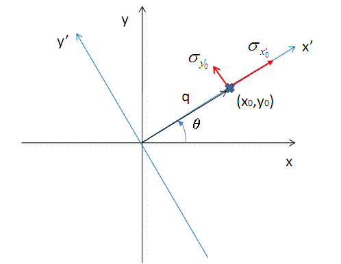
In Eq (9), x₀ = qcos(theta) and y₀=qsin(theta) , and the primed axes are in the coordinate rotated by an angle theta around z-axis (below) so that x’₀ =  x₀cos(theta) + y₀ sin(theta)  and y’₀ =  -x₀sin(theta) + y₀ cos(theta) . Note that the rotation angle is zero for x-y symmetric elliptical Gaussian distribution. The  A is a normalization factor.

Now we consider a numerical integration where each bins in THETA and R are evenly (this is to simplify the equation below) distributed by Delta_THETA and DeltaR, respectively, and it is assumed that I(x’, y’) is constant within the bins which in turn becomes

(10)

Since we have found the weighting factor on each bin points, it is convenient to transform x’-y’ back to x-y coordinate (rotating it by -(theta) around z axis).  Then, for the polar symmetric smear,

(11)

where,

while for the x-y symmetric smear,

                                                                                          (12)

where,

Here, the current version of the SANSVIEW uses the Eq. (11) for 2D smearing assuming that all the Gaussian weighting functions are aligned in the polar coordinate.

In the control panel, the higher accuracy indicates more and finer binnng points so that it costs more in time.