Model Functions

Introduction
Shapes: SphereModel, BinaryHSModel, FuzzySphereModel, CoreShellModel, CoreMultiShellModel, VesicleModel, MultiShellModel, OnionExpShellModel, SphericalSLDModel, PearlNecklaceModel , CylinderModel, CoreShellCylinderModel, HollowCylinderModel, FlexibleCylinderModel, FlexCylEllipXModel, StackedDisksModel, ParallelepipedModel, CSParallelepipedModel, EllipticalCylinderModel, BarBellModel, CappedCylinderModel, EllipsoidModel, CoreShellEllipsoidModel, TriaxialEllipsoidModel, LamellarModel, LamellarFFHGModel, LamellarPSModel, LamellarPSHGModel, LamellarPCrystalModel, SCCrystalModel, FCCrystalModel, BCCrystalModel.
Shape-Independent: AbsolutePower_Law, BEPolyelectrolyte, BroadPeak, CorrLength, DAB_Model, Debye, FractalModel, FractalCoreShell, GaussLorentzGel, Guinier, GuinierPorod, Lorentz, PeakGaussModel, PeakLorentzModel, Poly_GaussCoil, PolyExclVolume, PorodModel, RPA10Model, Teubner Strey, TwoLorentzian, TwoPowerLaw, UnifiedPowerRg, LineModel.
Customized Models: A+Bcos(2x)+Csin(2x), sin(poly)/(poly), Sum[P1(Cyl), P2(PEV)], ReflectivityModel, ReflectivityIIModel.
Structure Factors: HardSphereStructure, SquareWellStructure, HayterMSAStructure, StickyHSStructure.
References

The present text documents the modules made available by the DANSE software for SANS.

Readers are also referred to the SANS/DANSE wiki page:

http://danse.us/trac/sans

Note: Our model uses the form factor calculations implemented in a c-library provided by the NIST Center for Neutron Research and thus some content and figures in this document are originated from or shared with the NIST Igor analysis package by permission (S. Kline, NIST, 2006).

2. Shapes (Scattering Intensity Models)

This software provides form factors for various particle shapes. After giving a mathematical definition of each model, we draw the list of parameters available to the user. Validation plots for each model are also presented. Instructions on how to use the software is available with the source code, available from SVN:

svn co svn://danse.us/sans/releases/sansmodels-x.x

To easily compare to the scattering intensity measured in experiments, we normalize the form factors by the volume of the particle:

with

where P₀(q) is the un-normalized form factor, ρ(r) is the scattering length density at a given point in space and the integration is done over the volume V of the scatterer.

For systems without inter-particle interference, the form factors we provide can be related to the scattering intensity by the particle volume fraction: .

Our so-called 1D scattering intensity functions provide P(q) for the case where the scatterer is randomly oriented. In that case, the scattering intensity only depends on the length of q. The intensity measured on the plane of the SANS detector will have an azimuthal symmetry around q=0.

Our so-called 2D scattering intensity functions provide P(q, φ) for an oriented system as a function of a q-vector in the plane of the detector. We define the angle φ as the angle between the q vector and the horizontal (x) axis of the plane of the detector.

2.1. Sphere Model

This model provides the form factor, P(q), for a monodisperse spherical particle with uniform scattering length density. The form factor is normalized by the particle volume as described below.

1.1. Definition

The 1D scattering intensity is calculated in the following way (Guinier, 1955):

where scale is a scale factor* volume fraction, V is the volume of the scatterer, r is the radius of the sphere, bkg is the background level and sldXXX is the scattering length density (SLD) of the scatterer or the solvent.

Note that if your data is in absolute scale, the 'scale' should represent the volume fraction (unitless) if you have a good fit. If not, it should represent the volume fraction * a factor (by which your data might need to be rescaled).

The 2D scattering intensity is the same as P(q) above, regardless of the orientation of the q vector.

The returned value is scaled to units of [cm^-1] and the parameters of the sphere model are the following:

Parameter name	Units	Default value
scale	None	1
radius	Å	60
sldSph	Å^-2	2.0e-6
sldSolv	Å^-2	1.0e-6
background	cm^-1	0

Our model uses the form factor calculations implemented in a c-library provided by the NIST Center for Neutron Research (Kline, 2006).

2.1. Validation of the sphere model

Validation of our code was done by comparing the output of the 1D model to the output of the software provided by the NIST (Kline, 2006). Figure 1 shows a comparison of the output of our model and the output of the NIST software.

sphere_1D_validation

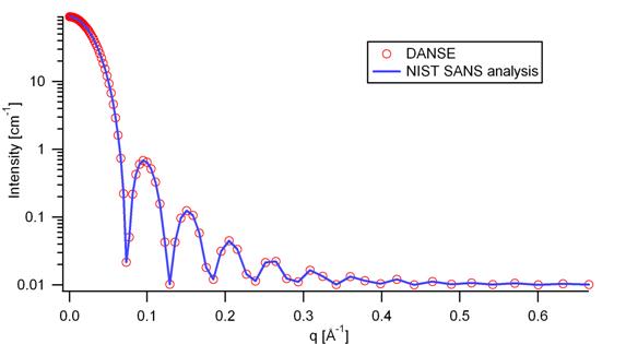
Figure 1: Comparison of the DANSE scattering intensity for a sphere with the output of the NIST SANS analysis software. The parameters were set to: Scale=1.0, Radius=60 Å, Contrast=1e-6 Å^-2, and Background=0.01 cm^-1.

2.2. BinaryHSModel

This model (binary hard sphere model) provides the scattering intensity, for binary mixture of spheres including hard sphere interaction between those particles. Using Percus-Yevick closure, the calculation is an exact multi-component solution:

where S_ij are the partial structure factors and f_i are the scattering amplitudes of the particles. And the subscript 1 is for the smaller particle and 2 is for the larger. The number fraction of the larger particle, (x = n₂/(n₁+n₂), n = the number density) is internally calculated based on:

The 2D scattering intensity is the same as 1D, regardless of the orientation of the q vector which is defined as.

The parameters of the binary hard sphere are the following (in the names, l (or ls) stands for larger spheres while s (or ss) for the smaller spheres):

Parameter name	Units	Default value
background	cm^-1	0.001
l_radius	Å	100.0
ss_sld	Å^-2	0.0
ls_sld	Å^-2	3e-6
solvent_sld	Å^-2	6e-6
s_radius	Å	25.0
vol_frac_ls	Å	0.1
vol_frac_ss	Å	0.2

Figure. 1D plot using the default values above (w/200 data point).

Our model uses the form factor calculations implemented in a c-library provided by the NIST Center for Neutron Research (Kline, 2006).

See the reference for details.

REFERENCE

N. W. Ashcroft and D. C. Langreth, Physical Review, v. 156 (1967) 685-692.

[Errata found in Phys. Rev. 166 (1968) 934.]

2.3. FuzzySphereModel

This model is to calculate the scattering from spherical particles with a "fuzzy" interface.

1.1. Definition

The 1D scattering intensity is calculated in the following way (Guinier, 1955):

The returned value is scaled to units of [cm-1 sr-1], absolute scale.

The scattering intensity I(q) is calculated as:

where the amplitude A(q) is given as the typical sphere scattering convoluted with a Gaussian to get a gradual drop-off in the scattering length density:

Here A²(q) is the form factor, P(q). The ‘scale’ is equivalent to the volume fraction of spheres, each of volume, V. Contrast (Δρ ) is the difference of scattering length densities of the sphere and the surrounding solvent.

The poly-dispersion in radius and in fuzziness is provided.

(direct from the reference)

The "fuzziness" of the interface is defined by the parameter (sigma)_fuzzy. The particle radius R represents the radius of the particle where the scattering length density profile decreased to 1/2 of the core density. The (sigma)_fuzzy is the width of the smeared particle surface: i.e., the standard deviation from the average height of the fuzzy interface. The inner regions of the microgel that display a higher density are described by the radial box profile extending to a radius of approximately Rbox ~ R - 2(sigma). the profile approaches zero as Rsans ~ R + 2(sigma).

For 2D data: The 2D scattering intensity is calculated in the same way as 1D, where the q vector is defined as.

REFERENCE

M. Stieger, J. S. Pedersen, P. Lindner, W. Richtering, Langmuir 20 (2004) 7283-7292.

TEST DATASET

This example dataset is produced by running the FuzzySphereModel, using 200 data points, qmin = 0.001 Å^-1, qmax = 0.7 A^-1 and the default values:

Parameter name	Units	Default value
scale	None	1.0
radius	Å	60
fuzziness	Å	10
sldSolv	Å^-2	3e-6
sldSph	Å^-2	1e-6
background	cm^-1	0.001

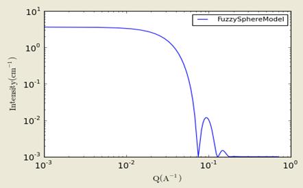
Figure. 1D plot using the default values (w/200 data point).

2.4. Core Shell (Sphere) Model

This model provides the form factor, P(q), for a spherical particle with a core-shell structure. The form factor is normalized by the particle volume.

1.1. Definition

The 1D scattering intensity is calculated in the following way (Guinier, 1955):

where scale is a scale factor, V_s is the volume of the outer shell, V_c is the volume of the core, r_s is the radius of the shell, r_c is the radius of the core, ρ_c is the scattering length density of the core, ρ_s is the scattering length density of the shell, ρ_solv is the scattering length density of the solvent, and bkg is the background level.

The 2D scattering intensity is the same as P(q) above, regardless of the orientation of the q vector.

For P*S: The outer most radius (= radius + thickness) is used as the effective radius toward S(Q) when P(Q)*S(Q) is applied.

The returned value is scaled to units of [cm^-1] and the parameters of the core-shell sphere model are the following:

Here, radius = the radius of the core and thickness = the thickness of the shell.

Parameter name	Units	Default value
scale	None	1.0
(core) radius	Å	60
thickness	Å	10
core_sld	Å^-2	1e-6
shell_sld	Å^-2	2e-6
solvent_sld	Å^-2	3e-6
background	cm^-1	0.001

Our model uses the form factor calculations implemented in a c-library provided by the NIST Center for Neutron Research (Kline, 2006).

REFERENCE

Guinier, A. and G. Fournet, "Small-Angle Scattering of X-Rays", John Wiley and Sons, New York, (1955).

2.1. Validation of the core-shell sphere model

core_shell_sphere_1D_validation

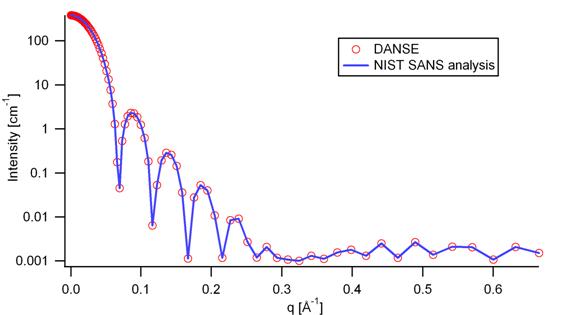
Figure 7: Comparison of the DANSE scattering intensity for a core-shell sphere with the output of the NIST SANS analysis software. The parameters were set to: Scale=1.0, Radius=60 Å, Contrast=1e-6 Å^-2, and Background=0.001 cm^-1.

2.5. CoreMultiShell(Sphere)Model

This model provides the scattering from spherical core with from 1 up to 4 shell structures. It has a core of a specified radius, with four shells. The SLDs of the core and each shell are individually specified.

1.1. Definition

The returned value is scaled to units of [cm-1sr-1], absolute scale.

This model is a trivial extension of the CoreShell function to a larger number of shells. See the CoreShell function for a diagram and documentation.

Be careful that the SLDs and scale can be highly correlated. Hold as many of these fixed as possible.

The 2D scattering intensity is the same as P(q) of 1D, regardless of the orientation of the q vector.

For P*S: The outer most radius (= radius + 4 thicknesses) is used as the effective radius toward S(Q) if P(Q)*S(Q) is applied.

The returned value is scaled to units of [cm^-1] and the parameters of the CoreFourshell sphere model are the following:

Here, rad_core = the radius of the core, thick_shelli = the thickness of the shell i and sld_shelli = the SLD of the shell i.

And the sld_core and the sld_solv are the SLD of the core and the solvent, respectively.

Parameter name	Units	Default value
scale	None	1.0
rad_core	Å	60
sld_core	Å^-2	6.4e-6
sld_shell1	Å^-2	1e-6
sld_shell2	Å^-2	2e-6
sld_shell3	Å^-2	3e-6
sld_shell4	Å^-2	4e-6
sld_solv	Å^-2	6.4e-6
thick_shell1	Å	10
thick_shell2	Å	10
thick_shell3	Å	10
thick_shell4	Å	10
background	cm^-1	0.001

Our model uses the form factor calculations implemented in a c-library provided by the NIST Center for Neutron Research (Kline, 2006).

REFERENCE

See the CoreShell documentation.

TEST DATASET

This example dataset is produced by running the CoreMultiShellModel using 200 data points, qmin = 0.001 Å-1, qmax = 0.7 Å-1 and the above default values.

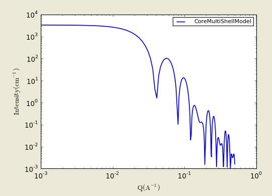
Figure: 1D plot using the default values (w/200 data point).

The scattering length density profile for the default sld values (w/ 4 shells).

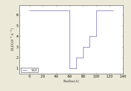
Figure: SLD profile against the radius of the sphere for default SLDs.

2.6. VesicleModel

This model provides the form factor, P(q), for an unilamellar vesicle. The form factor is normalized by the volume of the shell.

The 1D scattering intensity is calculated in the following way (Guinier, 1955):

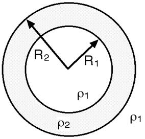
where scale is a scale factor, V_shell is the volume of the shell, V₁ is the volume of the core, V₂ is the total volume, R₁ is the radius of the core, r₂ is the outer radius of the shell, ρ₁ is the scattering length density of the core and the solvent, ρ₂ is the scattering length density of the shell, and bkg is the background level. And J₁ = (sinx - xcosx)/x². The functional form is identical to a "typical" core-shell structure, except that the scattering is normalized by the volume that is contributing to the scattering, namely the volume of the shell alone. Also, the vesicle is best defined in terms of a core radius (= R1) and a shell thickness, t.

The 2D scattering intensity is the same as P(q) above, regardless of the orientation of the q vector which is defined as.

For P*S: The outer most radius (= radius + thickness) is used as the effective radius toward S(Q) when P(Q)*S(Q) is applied.

The returned value is scaled to units of [cm^-1] and the parameters of the vesicle model are the following:

In the parameters, the ‘radius’ represents the core radius (R₁) and the ‘thickness’ (R₂ – R₁) is the shell thickness.

Parameter name	Units	Default value
scale	None	1.0
radius	Å	100
thickness	Å	30
core_sld	Å^-2	6.3e-6
shell_sld	Å^-2	0
background	cm^-1	0.0

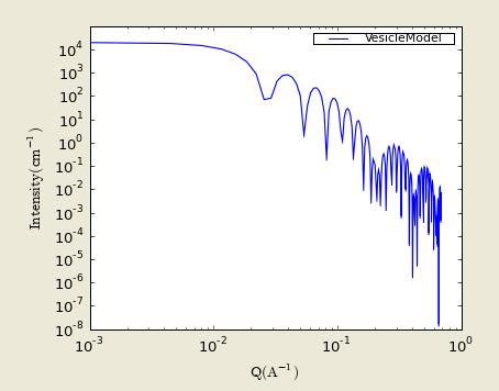
Figure. 1D plot using the default values (w/200 data point).

Our model uses the form factor calculations implemented in a c-library provided by the NIST Center for Neutron Research (Kline, 2006).

REFERENCE

Guinier, A. and G. Fournet, "Small-Angle Scattering of X-Rays", John Wiley and Sons, New York, (1955).

2.7. MultiShellModel

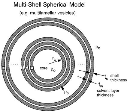
This model provides the form factor, P(q), for a multi-lamellar vesicle with N shells where the core is filled with solvent and the shells are interleaved with layers of solvent. For N = 1, this return to the vesicle model (above).

The 2D scattering intensity is the same as 1D, regardless of the orientation of the q vector which is defined as.

For P*S: The outer most radius (= core_radius + n_pairs * s_thickness + (n_pairs -1) * w_thickness) is used as the effective radius toward S(Q) when P(Q)*S(Q) is applied.

The returned value is scaled to units of [cm^-1] and the parameters of the multi-shell model are the following:

In the parameters, the ‘s_thickness’ is the shell thickness while the ‘w_thickness’ is the solvent thickness, and the n_pair is the number of shells.

Parameter name	Units	Default value
scale	None	1.0
core_radius	Å	60.0
n_pairs	None	2.0
core_sld	Å^-2	6.3e-6
shell_sld	Å^-2	0.0
background	cm^-1	0.0
s_thickness	Å	10
w_thickness	Å	10

Figure. 1D plot using the default values (w/200 data point).

Our model uses the form factor calculations implemented in a c-library provided by the NIST Center for Neutron Research (Kline, 2006).

REFERENCE

Cabane, B., Small Angle Scattering Methods, Surfactant Solutions: New Methods of Investigation, Ch.2, Surfactant Science Series Vol. 22, Ed. R. Zana, M. Dekker, New York, 1987.

2.8. OnionExpShellModel

This model provides the form factor, P(q), for a multi-shell sphere where the scattering length density (SLD) of the each shell is described by an exponential (linear, or flat-top) function. The form factor is normalized by the volume of the sphere where the SLD is not identical to the SLD of the solvent. We currently provide up to 9 shells with this model.

The 1D scattering intensity is calculated in the following way:

where, for a spherically symmetric particle with a particle density r(r) [L.A.Feigin and D.I.Svergun, ‘Structure Analysis by Small-Angle X-Ray and Neutron Scattering’, Plenum Press, New York, 1987],

so that

Here we assumed that the SLDs of the core and solvent are constant against r. Now let’s consider the SLD of a shell, r_shelli, defineded by

An example of a possible SLD profile is shown below where sld_in_shelli (r_in ) and thick_shelli (Dt_shelli ) stand for the SLD of the inner side of the i’th shell and the thickness of the i’th shell in the equation above, respectively.

For |A|>0,

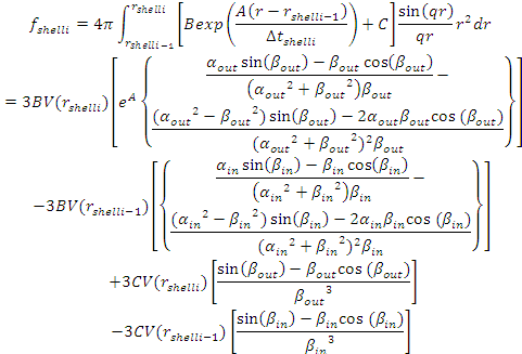
For A ~ 0 (eg., A = - 0.0001), this function converges to that of the linear SLD profile (ie, r_shelli(r) = A^’(r - r_shelli-1) /Dt_shelli) + B^’), so this case it is equivalent to

For A = 0, the exponential function has no dependence on the radius (so that ‘sld_out_shell#’ (r_out) is ignored this case) and becomes flat. We set the constant to r_in for convenience, and thus the form factor contributed by the shells is

In the equation,

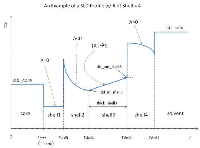
Finally, the form factor can be calculated by

where

The 2D scattering intensity is the same as P(q) above, regardless of the orientation of the q vector which is defined as.

For P*S: The outer most radius is used as the effective radius toward S(Q) when P(Q)*S(Q) is applied.

The returned value is scaled to units of [cm^-1] and the parameters of this model are the following:

In the parameters, the ‘rad_core’ represents the core radius (R₁) and the ‘thick_shell1’ (R₂ – R₁) is the thickness of the shell1, etc.

Note: Only No. of shells = 1 is given below.

Parameter name	Units	Default value
A_shell1	None	1
scale	None	1.0
rad_core	Å	200
thick_shell1	Å	50
sld_core	Å^-2	1.0e-06
sld_in_shell1	Å^-2	1.7e-06
sld_out_shell1	Å^-2	2.0e-06
sld_solv	Å^-2	6.4e-06
background	cm^-1	0.0

Figure. 1D plot using the default values (w/400 point).

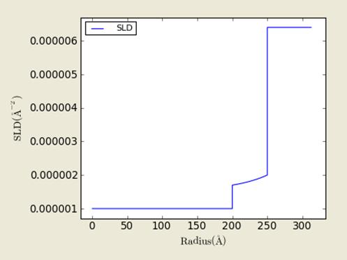
Figure. SLD profile from the default values.

REFERENCE

L.A.Feigin and D.I.Svergun, ‘Structure Analysis by Small-Angle X-Ray and Neutron Scattering’, Plenum Press, New York, 1987

2.9. SphericalSLDModel

Similarly to the OnionExpShellModel, this model provides the form factor, P(q), for a multi-shell sphere, where the interface between the each neighboring shells can be described by one of the functions including error, power-law, and exponential functions. This model is to calculate the scattering intensity by building a continuous custom SLD profile against the radius of the particle. The SLD profile is composed of a flat core, a flat solvent, a number (up to 9 shells) of flat shells, and the interfacial layers between the adjacent flat shells (or core, and solvent) (See below). Unlike OnionExpShellModel (using an analytical integration), the interfacial layers are sub-divided and numerically integrated assuming each sub-layers are described by a line function. The number of the sub-layer can be given by users by setting the integer values of ‘npts_inter#’ in GUI. The form factor is normalized by the total volume of the sphere.

The 1D scattering intensity is calculated in the following way:

so that

Here we assumed that the SLDs of the core and solvent are constant against r. The SLD at the interface between shells, r_{inter_i}, is calculated with a function chosen by an user, where the functions are:

1) Exp;

2) Power-Law;

3) Erf;

Then the functions are normalized so that it varies between 0 and 1 and they are constrained such that the SLD is continuous at the boundaries of the interface as well as each sub-layers and thus the B and C are determined.

Once the r_{inter_i} is found at the boundary of the sub-layer of the interface, we can find the its contribution to the form factor P(q);

where we assume that rho_inter_i (r) can be approximately linear within a sub-layer j.

In the equation,

Finally, the form factor can be calculated by

where

The 2D scattering intensity is the same as P(q) above, regardless of the orientation of the q vector which is defined as.

For P*S: The outer most radius is used as the effective radius toward S(Q) when P(Q)*S(Q) is applied.

The returned value is scaled to units of [cm^-1] and the parameters of this model are the following:

In the parameters, the ‘rad_core0’ represents the core radius (R₁).

Note: Only No. of shells = 1 is given below.

Parameter name	Units	Default value
background	cm^-1	0.0
npts_inter		35
scale		1
sld_solv	Å^-2	1e-006
func_inter1		Erf
nu_inter		2.5
thick_inter1	Å	50
sld_flat1	Å^-2	4e-006
thick_flat1	Å	100
func_inter0		Erf
nu_inter0		2.5
rad_core0	Å	50
sld_ core0	Å^-2	2.07e-06
thick_ core0	Å	50

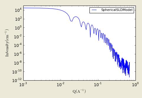
Figure. 1D plot using the default values (w/400 point).

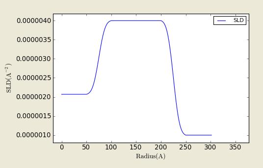
Figure. SLD profile from the default values.

REFERENCE

L.A.Feigin and D.I.Svergun, ‘Structure Analysis by Small-Angle X-Ray and Neutron Scattering’, Plenum Press, New York, 1987

2.10. PearlNecklaceModel

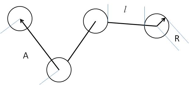
This model provides the form factor for a pearl necklace composed of two elements: N pearls (homogeneous spheres) freely jointed by M rods (like strings) (with a total mass M_w = M *m_r + N * m_s, the radius R and the string segment length (or edge separation) l (= A- 2R)). The A is the center to center pearl separation distance.

1.1. Definition

The output of the scattering intensity function for the pearlnecklace model is given by (Schweins, 2004):

where

and

where the mass m_i is (sld(of i) – sld(of solvent)) * (volume of the N pearls/rods), V is the total volume of the necklace.

The 2D scattering intensity is the same as P(q) above, regardless of the orientation of the q vector.

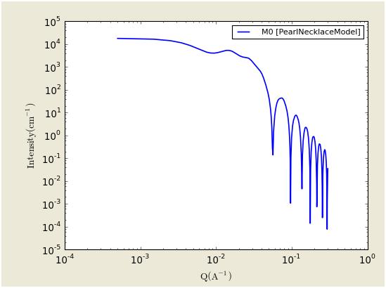
The returned value is scaled to units of [cm^-1] and the parameters of the sphere model are the following:

Parameter name	Units	Default value
scale	None	1.0
radius	Å	80.0
edge_separation	Å	350.0
num_pearls	(integer)	3
sld_pearl	Å^-2	1e-6
sld_solv	Å^-2	6.3e-6
sld_string	Å^-2	1e-6
thick_string (=rod diameter)	Å	2.5
background	cm^-1	0.0

REFERENCE

R. Schweins and K. Huber, ‘Particle Scattering Factor of Pearl Necklace Chains’, Macromol. Symp., 211, 25-42, 2004.

2.11. Cylinder Model

This model provides the form factor for a right circular cylinder with uniform scattering length density. The form factor is normalized by the particle volume.

1.1. Definition

The output of the 2D scattering intensity function for oriented cylinders is given by (Guinier, 1955):

where α is the angle between the axis of the cylinder and the q-vector, V is the volume of the cylinder, L is the length of the cylinder, r is the radius of the cylinder, and Δρ (contrast) is the scattering length density difference between the scatterer and the solvent. J₁ is the first order Bessel function.

To provide easy access to the orientation of the cylinder, we define the axis of the cylinder using two angles theta and phi. Those angles are defined on Figure 2.

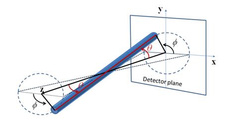
Figure 2a. Definition of the angles for oriented cylinders.

Figure 2b. Examples of the angles for oriented cylinders against the detector plane.

For P*S: The 2^nd virial coefficient of the cylinder is calculate based on the radius and length values, and used as the effective radius toward S(Q) when P(Q)*S(Q) is applied.

The returned value is scaled to units of [cm^-1] and the parameters of the cylinder model are the following:

Parameter name	Units	Default value
scale	None	1.0
radius	Å	20.0
length	Å	400.0
contrast	Å^-2	3.0e-6
background	cm^-1	0.0
cyl_theta	degree	60
cyl_phi	degree	60

The output of the 1D scattering intensity function for randomly oriented cylinders is then given by:

The cyl_theta and cyl_phi parameter are not used for the 1D output. Our implementation of the scattering kernel and the 1D scattering intensity use the c-library from NIST.

2.1. Validation of the cylinder model

Validation of our code was done by comparing the output of the 1D model to the output of the software provided by the NIST (Kline, 2006). Figure 3 shows a comparison of the 1D output of our model and the output of the NIST software.

In general, averaging over a distribution of orientations is done by evaluating the following:

where p(θ,φ) is the probability distribution for the orientation and P₀(q,α) is the scattering intensity for the fully oriented system. Since we have no other software to compare the implementation of the intensity for fully oriented cylinders, we can compare the result of averaging our 2D output using a uniform distribution p(θ,φ) = 1.0. Figure 4 shows the result of such a cross-check.

cylinder_1D_validation

Figure 3: Comparison of the DANSE scattering intensity for a cylinder with the output of the NIST SANS analysis software. The parameters were set to: Scale=1.0, Radius=20 Å, Length=400 Å, Contrast=3e-6 Å^-2, and Background=0.01 cm^-1.

cylinder_2D_average

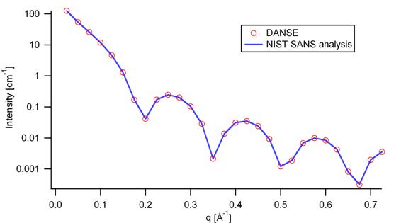
Figure 4: Comparison of the intensity for uniformly distributed cylinders calculated from our 2D model and the intensity from the NIST SANS analysis software. The parameters used were: Scale=1.0, Radius=20 Å, Length=400 Å, Contrast=3e-6 Å^-2, and Background=0.0 cm^-1.

2.12. Core-Shell Cylinder Model

This model provides the form factor for a circular cylinder with a core-shell scattering length density profile. The form factor is normalized by the particle volume.

1.1. Definition

The output of the 2D scattering intensity function for oriented core-shell cylinders is given by (Kline, 2006):

where α is the angle between the axis of the cylinder and the q-vector, V_s is the volume of the outer shell, V_c is the volume of the core, L is the length of the core, r is the radius of the core, t is the thickness of the shell, ρ_c is the scattering length density of the core, ρ_s is the scattering length density of the shell, ρ_solv is the scattering length density of the solvent, and bkg is the background level. The outer radius of the shell is given by r+t and the total length of the outer shell is given by L+2t. J₁ is the first order Bessel function.

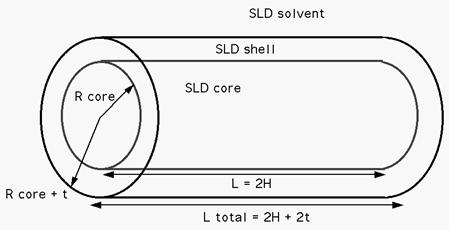
To provide easy access to the orientation of the core-shell cylinder, we define the axis of the cylinder using two angles θ and φ. Similarly to the case of the cylinder, those angles are defined on Figure 2 in Cylinder Model.

For P*S: The 2^nd virial coefficient of the solid cylinder is calculate based on the (radius+thickness) and 2(length +thickness) values, and used as the effective radius toward S(Q) when P(Q)*S(Q) is applied.

The returned value is scaled to units of [cm^-1] and the parameters of the core-shell cylinder model are the following:

Parameter name	Units	Default value
scale	None	1.0
radius	Å	20.0
thickness	Å	10.0
length	Å	400.0
core_sld	Å^-2	1e-6
shell_sld	Å^-2	4e-6
solvent_sld	Å^-2	1e-6
background	cm^-1	0.0
axis_theta	degree	90
axis_phi	degree	0.0

The output of the 1D scattering intensity function for randomly oriented cylinders is then given by the equation above.

The axis_theta and axis_phi parameters are not used for the 1D output. Our implementation of the scattering kernel and the 1D scattering intensity use the c-library from NIST.

2.1. Validation of the core-shell cylinder model

Validation of our code was done by comparing the output of the 1D model to the output of the software provided by the NIST (Kline, 2006). Figure 8 shows a comparison of the 1D output of our model and the output of the NIST software.

Averaging over a distribution of orientation is done by evaluating the equation above. Since we have no other software to compare the implementation of the intensity for fully oriented core-shell cylinders, we can compare the result of averaging our 2D output using a uniform distribution p(θ,φ) = 1.0. Figure 9 shows the result of such a cross-check.

core_shell_cylinder_1D_validation

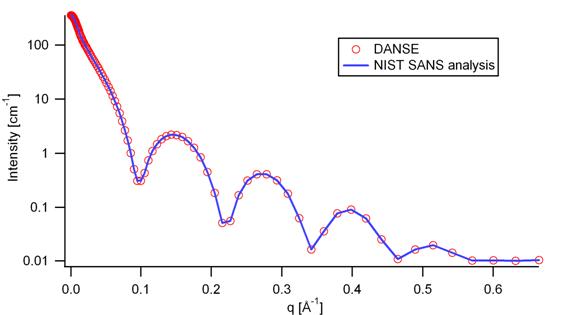
Figure 8: Comparison of the DANSE scattering intensity for a core-shell cylinder with the output of the NIST SANS analysis software. The parameters were set to: Scale=1.0, Radius=20 Å, Thickness=10 Å, Length=400 Å, Core_sld=1e-6 Å^-2, Shell_sld=4e-6 Å^-2, Solvent_sld=1e-6 Å^-2, and Background=0.01 cm^-1.

core_shell_cylinder_2D_average

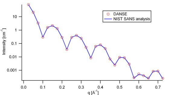
Figure 9: Comparison of the intensity for uniformly distributed core-shell cylinders calculated from our 2D model and the intensity from the NIST SANS analysis software. The parameters used were: Scale=1.0, Radius=20 Å, Thickness=10 Å, Length=400 Å, Core_sld=1e-6 Å^-2, Shell_sld=4e-6 Å^-2, Solvent_sld=1e-6 Å^-2, and Background=0.0 cm^-1.

2.13. HollowCylinderModel

This model provides the form factor, P(q), for a monodisperse hollow right angle circular cylinder (tube) where the form factor is normalized by the volume of the tube:

P(q) = scale*<f^2>/V_shell+background where the averaging < > id applied only for the 1D calculation. The inside and outside of the hollow cylinder have the same SLD.

The 1D scattering intensity is calculated in the following way (Guinier, 1955):

where scale is a scale factor, J₁ is the 1^st order Bessel function, J₁ (x)= (sinx - xcosx)/x².

For P*S: The 2^nd virial coefficient of the solid cylinder is calculate based on the (radius) and 2(length) values, and used as the effective radius toward S(Q) when P(Q)*S(Q) is applied.

In the parameters, the ‘contrast’ represents SLD (shell) - SLD (solvent) and the radius = R_hell while core_radius = R_core.

Parameter name	Units	Default value
scale	None	1.0
radius	Å	30
length	Å	400
core_radius	Å	20
sldCyl	Å^-2	6.3e-6
sldSolv	Å^-2	5e-06
background	cm^-1	0.01

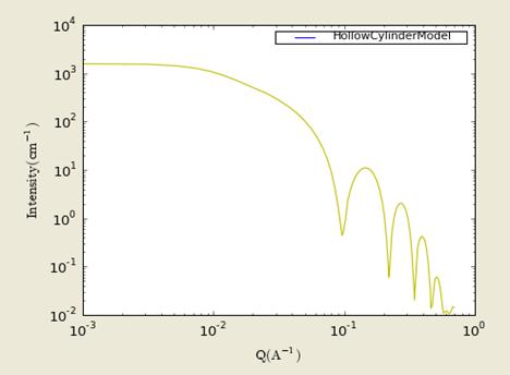
Figure. 1D plot using the default values (w/1000 data point).

Our model uses the form factor calculations implemented in a c-library provided by the NIST Center for Neutron Research (Kline, 2006).

REFERENCE

Feigin, L. A, and D. I. Svergun, "Structure Analysis by Small-Angle X-Ray and Neutron Scattering", Plenum Press, New York, (1987).

2.14. FlexibleCylinderModel

This model provides the form factor, P(q), for a flexible cylinder where the form factor is normalized by the volume of the cylinder: Inter-cylinder interactions are NOT included. P(q) = scale*<f^2>/V+background where the averaging < > is applied over all orientation for 1D. The 2D scattering intensity is the same as 1D, regardless of the orientation of the q vector which is defined as.

The chain of contour length, L, (the total length) can be described a chain of some number of locally stiff segments of length lp. The persistence length,lp, is the length along the cylinder over which the flexible cylinder can be considered a rigid rod. The Kuhn length (b = 2*lp) is also used to describe the stiffness of a chain. The returned value is in units of [cm-1], on absolute scale. In the parameters, the sldCyl and sldSolv represent SLD (chain/cylinder) and SLD (solvent) respectively.

Parameter name	Units	Default value
scale	None	1.0
radius	Å	20
length	Å	1000
sldCyl	Å^-2	1e-06
sldSolv	Å^-2	6.3e-06
background	cm^-1	0.01
kuhn_length	Å	100

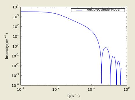
Figure. 1D plot using the default values (w/1000 data point).

Our model uses the form factor calculations implemented in a c-library provided by the NIST Center for Neutron Research (Kline, 2006):

From the reference, "Method 3 With Excluded Volume" is used. The model is a parametrization of simulations of a discrete representation of the worm-like chain model of Kratky and Porod applied in the pseudocontinuous limit. See equations (13,26-27) in the original reference for the details.

REFERENCE

Pedersen, J. S. and P. Schurtenberger (1996). “Scattering functions of semiflexible polymers with and without excluded volume effects.” Macromolecules 29: 7602-7612.

Correction of the formula can be found in:

Wei-Ren Chen, Paul D. Butler, and Linda J. Magid, "Incorporating Intermicellar Interactions in the Fitting of SANS Data from Cationic Wormlike Micelles" Langmuir, August 2006.

2.15. FlexCylEllipXModel

Flexible Cylinder with Elliptical Cross-Section: Calculates the form factor for a flexible cylinder with an elliptical cross section and a uniform scattering length density. The non-negligible diameter of the cylinder is included by accounting for excluded volume interactions within the walk of a single cylinder. The form factor is normalized by the particle volume such that P(q) = scale*<f^2>/Vol + bkg, where < > is an average over all possible orientations of the flexible cylinder.

1.1. Definition

The function calculated is from the reference given below. From that paper, "Method 3 With Excluded Volume" is used. The model is a parameterization of simulations of a discrete representation of the worm-like chain model of Kratky and Porod applied in the pseudo-continuous limit. See equations (13, 26-27) in the original reference for the details.

NOTE: there are several typos in the original reference that have been corrected by WRC. Details of the corrections are in the reference below.

- Equation (13): the term (1-w(QR)) should swap position with w(QR)

- Equations (23) and (24) are incorrect. WRC has entered these into Mathematica and solved analytically. The results were converted to code.

- Equation (27) should be q0 = max(a3/sqrt(RgSquare),3) instead of max(a3*b/sqrt(RgSquare),3)

- The scattering function is negative for a range of parameter values and q-values that are experimentally accessible. A correction function has been added to give the proper behavior.

The chain of contour length, L, (the total length) can be described a chain of some number of locally stiff segments of length lp. The persistence length, lp, is the length along the cylinder over which the flexible cylinder can be considered a rigid rod. The Kuhn length (b) used in the model is also used to describe the stiffness of a chain, and is simply b = 2*lp.

The cross section of the cylinder is elliptical, with minor radius a. The major radius is larger, so of course, the axis ratio (parameter 4) must be greater than one. Simple constraints should be applied during curve fitting to maintain this inequality.

The returned value is in units of [cm-1], on absolute scale.

The sldCyl = SLD (chain), sldSolv = SLD (solvent). The ‘scale’, and the contrast are both multiplicative factors in the model and are perfectly correlated. One or both of these parameters must be held fixed during model fitting.

If the ‘scale’ is set equal to the particle volume fraction, f, the returned value is the scattered intensity per unit volume, I(q) = f*P(q). However, no inter-particle interference effects are included in this calculation.

For 2D data: The 2D scattering intensity is calculated in the same way as 1D, where the q vector is defined as.

REFERENCE

Pedersen, J. S. and P. Schurtenberger (1996). “Scattering functions of semiflexible polymers with and without excluded volume effects.” Macromolecules 29: 7602-7612.

Corrections are in:

Wei-Ren Chen, Paul D. Butler, and Linda J. Magid, "Incorporating Intermicellar Interactions in the Fitting of SANS Data from Cationic Wormlike Micelles" Langmuir, August 2006.

TEST DATASET

This example dataset is produced by running the Macro FlexCylEllipXModel, using 200 data points, qmin = 0.001 Å-1, qmax = 0.7 Å-1 and the default values below.

Parameter name	Units	Default value
axis_ratio		1.5
background	cm^-1	0.0001
Kuhn_length	Å	100
(Contour) length	Å	1e+3
radius	Å	20.0
scale		1.0
sldCyl	Å^-2	1e-6
sldSolv	Å^-2	6.3e-6

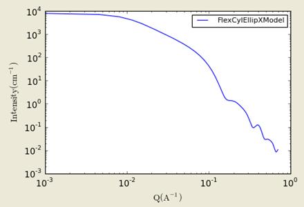
Figure. 1D plot using the default values (w/200 data points).

2.16. StackedDisksModel

This model provides the form factor, P(q), for stacked discs (tactoids) with a core/layer structure where the form factor is normalized by the volume of the cylinder. Assuming the next neighbor distance (d-spacing) in a stack of parallel discs obeys a Gaussian distribution, a structure factor S(q) proposed by Kratky and Porod in 1949 is used in this function. Note that the resolution smearing calculation uses 76 Gauss quadrature points to properly smear the model since the function is HIGHLY oscillatory, especially around the q-values that correspond to the repeat distance of the layers.

The 2D scattering intensity is the same as 1D, regardless of the orientation of the q vector which is defined as.

The returned value is in units of [cm^-1 sr^-1], on absolute scale.

The scattering intensity I(q) is:

where the contrast,

N is the number of discs per unit volume, a is the angle between the axis of the disc and q, and Vt and Vc are the total volume and the core volume of a single disc, respectively.

where d = thickness of the layer (layer_thick), 2h= core thickness (core_thick), and R = radius of the disc (radius).

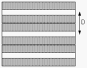
where n = the total number of the disc stacked (n_stacking), D=the next neighbor center to cent distance (d-spacing), and s_D = the Gaussian standard deviation of the d-spacing (sigma_d).

To provide easy access to the orientation of the stackeddisks, we define the axis of the cylinder using two angles θ and φ. Similarly to the case of the cylinder, those angles are defined on Figure 2 of CylinderModel.

For P*S: The 2^nd virial coefficient of the solid cylinder is calculate based on the (radius) and length = n_stacking*(core_thick +2*layer_thick) values, and used as the effective radius toward S(Q) when P(Q)*S(Q) is applied.

Parameter name	Units	Default value
background	cm^-1	0.001
core_sld	Å^-2	4e-006
core_thick	Å	10
layer_sld	Å^-2	0
layer_thick	Å	15
n_stacking		1
radius	Å	3e+003
scale		0.01
sigma_d		0
solvent_sld	Å^-2	5e-006

Figure. 1D plot using the default values (w/1000 data point).

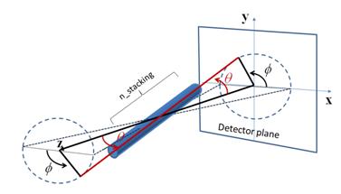
Figure. Examples of the angles for oriented stackeddisks against the detector plane.

Our model uses the form factor calculations implemented in a c-library provided by the NIST Center for Neutron Research (Kline, 2006):

REFERENCE

Guinier, A. and Fournet, G., "Small-Angle Scattering of X-Rays", John Wiley and Sons, New York, 1955.

Kratky, O. and Porod, G., J. Colloid Science, 4, 35, 1949.

Higgins, J.S. and Benoit, H.C., "Polymers and Neutron Scattering", Clarendon, Oxford, 1994.

2.17. ParallelepipedModel

This model provides the form factor, P(q), for a rectangular cylinder (below) where the form factor is normalized by the volume of the cylinder. P(q) = scale*<f^2>/V+background where the volume V= ABC and the averaging < > is applied over all orientation for 1D.

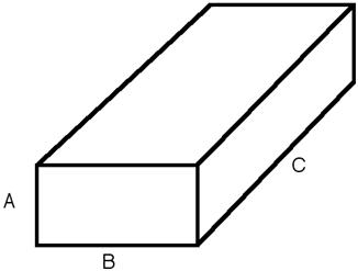
The side of the solid must be satisfied the condition of A<B<C in order for the calculation to be correct: where A = short_a, B=short_b, and C=long_c for the fitting parameters.

By this definition, assuming

a = A/B<1; b=B/B=1; c=C/B>1, the form factor,

The contrast is defined as

The scattering intensity per unit volume is returned in the unit of [cm^-1]; I(q) = fP(q).

For P*S: The 2^nd virial coefficient of the solid cylinder is calculate based on the averaged effective radius (= sqrt(short_a*short_b/pi)) and length( = long_c) values, and used as the effective radius toward S(Q) when P(Q)*S(Q) is applied.

To provide easy access to the orientation of the parallelepiped, we define the axis of the cylinder using two angles θ , φ and Y . Similarly to the case of the cylinder, those angles, θ and φ, are defined on Figure 2 of CylinderModel. The angle Y is the rotational angle around its own long_c axis against the q plane. For example, Y = 0 when the short_b axis is parallel to the x-axis of the detector.

Figure. Definition of angles for 2D.

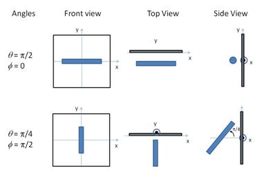
Figure. Examples of the angles for oriented pp against the detector plane.

Parameter name	Units	Default value
background	cm^-1	0.0
contrast	Å^-2	5e-006
long_c	Å	400
short_a	Å^-2	35
short_b	Å	75
scale		1

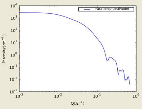
Figure. 1D plot using the default values (w/1000 data point).

· Validation of the parallelepiped 2D model

Validation of our code was done by comparing the output of the 1D calculation to the angular average of the output of 2 D calculation over all possible angles. The Figure below shows the comparison where the solid dot refers to averaged 2D while the line represents the result of 1D calculation (for the averaging, 76, 180, 76 points are taken over the angles of theta, phi, and psi respectively).

Figure. Comparison between 1D and averaged 2D.

Our model uses the form factor calculations implemented in a c-library provided by the NIST Center for Neutron Research (Kline, 2006):

REFERENCE

Mittelbach and Porod, Acta Physica Austriaca 14 (1961) 185-211.

Equations (1), (13-14). (in German)

2.18. CSParallelepipedModel

Calculates the form factor for a rectangular solid with a core-shell structure. The thickness and the scattering length density of the shell or "rim" can be different on all three (pairs) of faces. The form factor is normalized by the particle volume such that P(q) = scale*<f^2>/Vol + bkg, where < > is an average over all possible orientations of the rectangular solid. An instrument resolution smeared version is also provided.

The function calculated is the form factor of the rectangular solid below. The core of the solid is defined by the dimensions ABC such that A < B < C.

There are rectangular "slabs" of thickness tA that add to the A dimension (on the BC faces). There are similar slabs on the AC (=tB) and AB (=tC) faces. The projection in the AB plane is then:

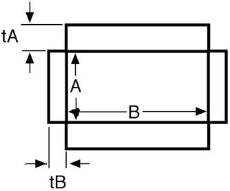
The volume of the solid is:

meaning that there are "gaps" at the corners of the solid.

The intensity calculated follows the parallelepiped model, with the core-shell intensity being calculated as the square of the sum of the amplitudes of the core and shell, in the same manner as a core-shell sphere.

For the calculation of the form factor to be valid, the sides of the solid MUST be chosen such that A < B < C. If this inequality in not satisfied, the model will not report an error, and the calculation will not be correct.

FITTING NOTES:

If the scale is set equal to the particle volume fraction, f, the returned value is the scattered intensity per unit volume, I(q) = f*P(q). However, no interparticle interference effects are included in this calculation.

There are many parameters in this model. Hold as many fixed as possible with known values, or you will certainly end up at a solution that is unphysical.

Constraints must be applied during fitting to ensure that the inequality A < B < C is not violated. The calculation will not report an error, but the results will not be correct.

The returned value is in units of [cm-1], on absolute scale.

For P*S: The 2^nd virial coefficient of this CSPP is calculate based on the averaged effective radius (= sqrt((short_a+2*rim_a)*(short_b+2*rim_b)/pi)) and length( = long_c+2*rim_c) values, and used as the effective radius toward S(Q) when P(Q)*S(Q) is applied.

To provide easy access to the orientation of the CSparallelepiped, we define the axis of the cylinder using two angles θ , φ and Y . Similarly to the case of the cylinder, those angles, θ and φ, are defined on Figure 2 of CylinderModel. The angle Y is the rotational angle around its own long_c axis against the q plane. For example, Y = 0 when the short_b axis is parallel to the x-axis of the detector.

Figure. Definition of angles for 2D.

Figure. Examples of the angles for oriented cspp against the detector plane.

TEST DATASET

This example dataset is produced by running the Macro Plot_CSParallelepiped(), using 100 data points, qmin = 0.001 Å-1, qmax = 0.7 Å-1 and the below default values.

Parameter name	Units	Default value
background	cm^-1	0.06
sld_pcore	Å^-2	1e-006
sld_rimA	Å^-2	2e-006
sld_rimB	Å^-2	4e-006
sld_rimC	Å^-2	2e-006
sld_solv	Å^-2	6e-006
rimA	Å	10
rimB	Å	10
rimC	Å	10
longC	Å	400
shortA	Å	35
midB	Å	75
scale		1

Figure. 1D plot using the default values (w/256 data points).

Figure. 2D plot using the default values (w/(256X265) data points).

Our model uses the form factor calculations implemented in a c-library provided by the NIST Center for Neutron Research (Kline, 2006):

REFERENCE

see: Mittelbach and Porod, Acta Physica Austriaca 14 (1961) 185-211.

Equations (1), (13-14). (yes, it's in German)

2.19. Elliptical Cylinder Model

This function calculates the scattering from an oriented elliptical cylinder.

For 2D (orientated system):

The angles theta and phi define the orientation of the axis of the cylinder. The angle psi is defined as the orientation of the major axis of the ellipse with respect to the vector Q. A gaussian poydispersity can be added to any of the orientation angles, and also for the minor radius and the ratio of the ellipse radii.

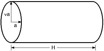
Figure. a= r_minor and n= r_ratio (i.e., r_major/r_minor).

The function calculated is:

with the functions:

(13)

and the angle psi is defined as the orientation of the major axis of the ellipse with respect to the vector Q.

For 1D (no preferred orientation):

The form factor is averaged over all possible orientation before normalized by the particle volume: P(q) = scale*<f^2>/V .

The returned value is scaled to units of [cm^-1].

To provide easy access to the orientation of the elliptical, we define the axis of the cylinder using two angles θ , φ and Y . Similarly to the case of the cylinder, those angles, θ and φ, are defined on Figure 2 of CylinderModel. The angle Y is the rotational angle around its own long_c axis against the q plane. For example, Y = 0 when the r_minor axis is parallel to the x-axis of the detector.

All angle parameters are valid and given only for 2D calculation (Oriented system).

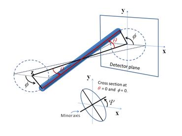
Figure. Definition of angels for 2D.

Figure. Examples of the angles for oriented elliptical cylinders

against the detector plane.

For P*S: The 2^nd virial coefficient of the solid cylinder is calculate based on the averaged radius (=sqrt(r_minor^2*r_ratio)) and length values, and used as the effective radius toward S(Q) when P(Q)*S(Q) is applied.

Parameter name	Units	Default value
scale	None	1.0
r_minor	Å	20.0
r_ratio	Å	1.5
length	Å	400.0
sldCyl	Å^-2	4e-6
sldSolv	Å^-2	1e-006
background		0

Figure. 1D plot using the default values (w/1000 data point).

· Validation of the elliptical cylinder 2D model

Validation of our code was done by comparing the output of the 1D calculation to the angular average of the output of 2 D calculation over all possible angles. The Figure below shows the comparison where the solid dot refers to averaged 2D while the line represents the result of 1D calculation (for 2D averaging, 76, 180, 76 points are taken for the angles of theta, phi, and psi respectively).

Figure. Comparison between 1D and averaged 2D.

In the 2D average, more binning in the angle phi is necessary to get the proper result. The following figure shows the results of the averaging by varying the number of bin over angles.

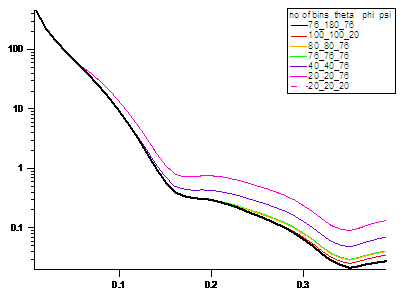
Figure. The intensities averaged from 2D over different number

of points of binning of angles.

REFERENCE

L. A. Feigin and D. I. Svergun “Structure Analysis by Small-Angle X-Ray and Neutron Scattering”, Plenum, New York, (1987).

2.20. BarBell(/DumBell)Model

Calculates the scattering from a barbell-shaped cylinder (This model simply becomes the DumBellModel when the length of the cylinder, L, is set to zero). That is, a sphereocylinder with spherical end caps that have a radius larger than that of the cylinder and the center of the end cap radius lies outside of the cylinder All dimensions of the barbell are considered to be monodisperse. See the diagram for the details of the geometry and restrictions on parameter values.

1.1. Definition

The returned value is scaled to units of [cm-1sr-1], absolute scale.

The barbell geometry is defined as:

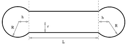
r is the radius of the cylinder. All other parameters are as defined in the diagram. Since the end cap radius R >= r and by definition for this geometry h > 0, h is then defined by r and R as:

h = sqrt(R^2 - r^2).

The scattering intensity I(q) is calculated as:

where the amplitude A(q) is given as:

The < > brackets denote an average of the structure over all orientations. <A^2(q)> is then the form factor, P(q). The scale factor is equivalent to the volume fraction of cylinders, each of volume, V. Contrast is the difference of scattering length densities of the cylinder and the surrounding solvent.

The volume of the barbell is:

and its radius of gyration:

The necessary conditions of R >= r is not enforced in the model. It is up to you to restrict this during analysis.

REFERENCES

H. Kaya, J. Appl. Cryst. (2004) 37, 223-230.

H. Kaya and N-R deSouza, J. Appl. Cryst. (2004) 37, 508-509. (addenda and errata)

TEST DATASET

This example dataset is produced by running the Macro PlotBarbell(), using 200 data points, qmin = 0.001 Å-1, qmax = 0.7 Å-1 and the above default values.

Parameter name	Units	Default value
scale	None	1.0
len_bar	Å	400.0
rad_bar	Å	20.0
rad_bell	Å	40.0
sld_barbell	Å^-2	1.0e-006
sld_solv	Å^-2	6.3e-006
background		0

Figure. 1D plot using the default values (w/256 data point).

For 2D data: The 2D scattering intensity is calculated similar to the 2D cylinder model. At the theta = 45 deg and phi =0 deg with default values for other parameters,

Figure. 2D plot (w/(256X265) data points).

2.21. CappedCylinder(/ConvexLens)Model

Calculates the scattering from a cylinder with spherical section end-caps(This model simply becomes the ConvexLensModel when the length of the cylinder L = 0. That is, a sphereocylinder with end caps that have a radius larger than that of the cylinder and the center of the end cap radius lies within the cylinder. See the diagram for the details of the geometry and restrictions on parameter values.

1.1. Definition

The returned value is scaled to units of [cm-1sr-1], absolute scale.

The Capped Cylinder geometry is defined as:

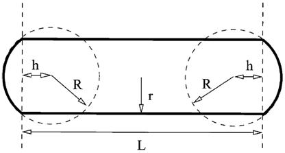
r is the radius of the cylinder. All other parameters are as defined in the diagram. Since the end cap radius R >= r and by definition for this geometry h < 0, h is then defined by r and R as:

h = -1*sqrt(R^2 - r^2).

The scattering intensity I(q) is calculated as:

where the amplitude A(q) is given as:

The volume of the Capped Cylinder is:

(with h as a positive value here)

and its radius of gyration:

The necessary conditions of R >= r is not enforced in the model. It is up to you to restrict this during analysis.

REFERENCES

H. Kaya, J. Appl. Cryst. (2004) 37, 223-230.

H. Kaya and N-R deSouza, J. Appl. Cryst. (2004) 37, 508-509. (addenda and errata)

TEST DATASET

This example dataset is produced by running the Macro CappedCylinder(), using 200 data points, qmin = 0.001 Å-1, qmax = 0.7 Å-1 and the above default values.

Parameter name	Units	Default value
scale	None	1.0
len_cyl	Å	400.0
rad_cap	Å	40.0
rad_cyl	Å	20.0
sld_capcyl	Å^-2	1.0e-006
sld_solv	Å^-2	6.3e-006
background		0

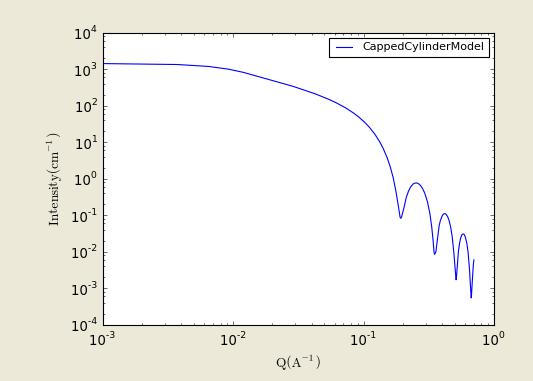
Figure. 1D plot using the default values (w/256 data point).

For 2D data: The 2D scattering intensity is calculated similar to the 2D cylinder model. At the theta = 45 deg and phi =0 deg with default values for other parameters,

Figure. 2D plot (w/(256X265) data points).

2.22. Ellipsoid Model

This model provides the form factor for an ellipsoid (ellipsoid of revolution) with uniform scattering length density. The form factor is normalized by the particle volume.

1.1. Definition

The output of the 2D scattering intensity function for oriented ellipsoids is given by (Feigin, 1987):

where α is the angle between the axis of the ellipsoid and the q-vector, V is the volume of the ellipsoid, R_a is the radius along the rotation axis of the ellipsoid, R_b is the radius perpendicular to the rotation axis of the ellipsoid and Δρ (contrast) is the scattering length density difference between the scatterer and the solvent.

To provide easy access to the orientation of the ellipsoid, we define the rotation axis of the ellipsoid using two angles θ and φ. Similarly to the case of the cylinder, those angles are defined on Figure 2. For the ellipsoid, θ is the angle between the rotation axis and the z-axis.

For P*S: The 2^nd virial coefficient of the solid ellipsoid is calculate based on the radius_a and radius_b values, and used as the effective radius toward S(Q) when P(Q)*S(Q) is applied.

The returned value is scaled to units of [cm^-1] and the parameters of the ellipsoid model are the following:

Parameter name	Units	Default value
scale	None	1.0
radius_a (polar)	Å	20.0
radius_b (equatorial)	Å	400.0
sldEll	Å^-2	4.0e-6
sldSolv	Å^-2	1.0e-6
background	cm^-1	0.0
axis_theta	degree	90
axis_phi	degree	0.0

The output of the 1D scattering intensity function for randomly oriented ellipsoids is then given by the equation above.

The axis_theta and axis_phi parameters are not used for the 1D output. Our implementation of the scattering kernel and the 1D scattering intensity use the c-library from NIST.

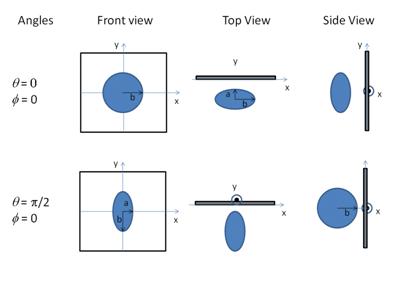
Figure. Examples of the angles for oriented ellipsoid

against the detector plane.

2.1. Validation of the ellipsoid model

Validation of our code was done by comparing the output of the 1D model to the output of the software provided by the NIST (Kline, 2006). Figure 5 shows a comparison of the 1D output of our model and the output of the NIST software.

Averaging over a distribution of orientation is done by evaluating the equation above. Since we have no other software to compare the implementation of the intensity for fully oriented ellipsoids, we can compare the result of averaging our 2D output using a uniform distribution p(θ,φ) = 1.0. Figure 6 shows the result of such a cross-check.

The discrepancy above q=0.3 Å^-1 is due to the way the form factors are calculated in the c-library provided by NIST. A numerical integration has to be performed to obtain P(q) for randomly oriented particles. The NIST software performs that integration with a 76-point Gaussian quadrature rule, which will become imprecise at high q where the amplitude varies quickly as a function of q. The DANSE result shown has been obtained by summing over 501 equidistant points in α. Our result was found to be stable over the range of q shown for a number of points higher than 500.

Figure 5: Comparison of the DANSE scattering intensity for an ellipsoid with the output of the NIST SANS analysis software. The parameters were set to: Scale=1.0, Radius_a=20 Å, Radius_b=400 Å,

Contrast=3e-6 Å^-2, and Background=0.01 cm^-1.

ellipsoid_2D_average

Figure 6: Comparison of the intensity for uniformly distributed ellipsoids calculated from our 2D model and the intensity from the NIST SANS analysis software. The parameters used were: Scale=1.0, Radius_a=20 Å, Radius_b=400 Å, Contrast=3e-6 Å^-2, and Background=0.0 cm^-1.

2.23. CoreShellEllipsoidModel

This model provides the form factor, P(q), for a core shell ellipsoid (below) where the form factor is normalized by the volume of the cylinder. P(q) = scale*<f^2>/V+background where the volume V= 4pi/3*r_maj*r_min² and the averaging < > is applied over all orientation for 1D.

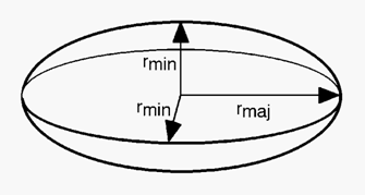
The returned value is in units of [cm^-1], on absolute scale.

The form factor calculated is:

To provide easy access to the orientation of the coreshell ellipsoid, we define the axis of the solid ellipsoid using two angles θ , φ. Similarly to the case of the cylinder, those angles, θ and φ, are defined on Figure 2 of CylinderModel.

The contrast is defined as SLD(core) – SLD(shell) or SLD(shell – solvent). In the parameters, equat_core = equatorial radius of the core, polar_core = polar radius of the core, equat_shell = r_min (or equatorial radius of the shell), and polar_shell = = r_maj (or polar radius of the shell).

For P*S: The 2^nd virial coefficient of the solid ellipsoid is calculate based on the radius_a (= polar_shell) and radius_b (= equat_shell) values, and used as the effective radius toward S(Q) when P(Q)*S(Q) is applied.

Parameter name	Units	Default value
background	cm^-1	0.001
equat_core	Å	200
equat_shell	Å	250
sld_solvent	Å^-2	6e-006
ploar_shell	Å	30
ploar_core	Å	20
scale		1
sld_core	Å^-2	2e-006
sld_shell	Å^-2	1e-006

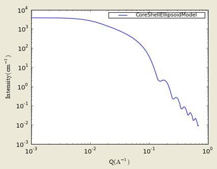
Figure. 1D plot using the default values (w/1000 data point).

Figure. Examples of the angles for oriented coreshellellipsoid against the detector plane where a =polar axis.

Our model uses the form factor calculations implemented in a c-library provided by the NIST Center for Neutron Research (Kline, 2006):

REFERENCE

Kotlarchyk, M.; Chen, S.-H. J. Chem. Phys., 1983, 79, 2461.

Berr, S. J. Phys. Chem., 1987, 91, 4760.

2.24. TriaxialEllipsoidModel

This model provides the form factor, P(q), for an ellipsoid (below) where all three axes are of different lengths, i.e., R_a =< R_b =< R_c (Note that users should maintains this inequality for the all calculations). P(q) = scale*<f^2>/V+background where the volume V= 4pi/3*R_a*R_b*R_c, and the averaging < > is applied over all orientation for 1D.

The returned value is in units of [cm^-1], on absolute scale.

The form factor calculated is:

To provide easy access to the orientation of the triaxial ellipsoid, we define the axis of the cylinder using the angles θ , φ and Y . Similarly to the case of the cylinder, those angles, θ and φ, are defined on Figure 2 of CylinderModel. The angle Y is the rotational angle around its own semi_axisC axis against the q plane. For example, Y = 0 when the semi_axisA axis is parallel to the x-axis of the detector.

The radius of gyration for this system is R_g² = (R_a²*R_b²*R_c²)/5. The contrast is defined as SLD(ellipsoid) – SLD(solvent). In the parameters, semi_axisA = R_a (or minor equatorial radius), semi_axisB = R_b (or major equatorial radius), and semi_axisC = R_c (or polar radius of the ellipsoid).

For P*S: The 2^nd virial coefficient of the solid ellipsoid is calculate based on the radius_a (=semi_axisC) and radius_b (=sqrt(semi_axisA* semi_axisB)) values, and used as the effective radius toward S(Q) when P(Q)*S(Q) is applied.

Parameter name	Units	Default value
background	cm^-1	0.0
semi_axisA	Å	35
semi_axisB	Å	100
semi_axisC	Å	400
scale		1
sldEll	Å^-2	1.0e-006
sldSolv	Å^-2	6.3e-006

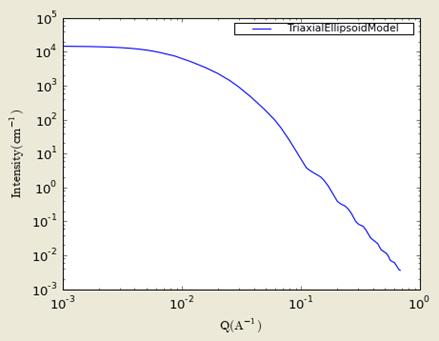
Figure. 1D plot using the default values (w/1000 data point).

· Validation of the triaxialellipsoid 2D model

Validation of our code was done by comparing the output of the 1D calculation to the angular average of the output of 2 D calculation over all possible angles. The Figure below shows the comparison where the solid dot refers to averaged 2D while the line represents the result of 1D calculation (for 2D averaging, 76, 180, 76 points are taken for the angles of theta, phi, and psi respectively).

Figure. Comparison between 1D and averaged 2D.

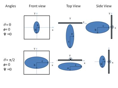
Figure. Examples of the angles for oriented ellipsoid against the detector plane.

Our model uses the form factor calculations implemented in a c-library provided by the NIST Center for Neutron Research (Kline, 2006):

REFERENCE

L. A. Feigin and D. I. Svergun “Structure Analysis by Small-Angle X-Ray and Neutron Scattering”, Plenum, New York, 1987.

2.25. LamellarModel

This model provides the scattering intensity, I(q), for a lyotropic lamellar phase where a uniform SLD and random distribution in solution are assumed. The ploydispersion in the bilayer thickness can be applied from the GUI.

The scattering intensity I(q) is:

The form factor is,

where d = bilayer thickness.

The 2D scattering intensity is calculated in the same way as 1D, where the q vector is defined as.

The returned value is in units of [cm^-1], on absolute scale. In the parameters, sld_bi = SLD of the bilayer, sld_sol = SLD of the solvent, and bi_thick = the thickness of the bilayer.

Parameter name	Units	Default value
background	cm^-1	0.0
sld_bi	Å^-2	1e-006
bi_thick	Å	50
sld_sol	Å^-2	6e-006
scale		1

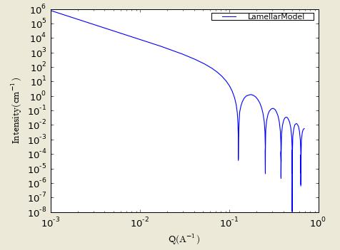
Figure. 1D plot using the default values (w/1000 data point).

Our model uses the form factor calculations implemented in a c-library provided by the NIST Center for Neutron Research (Kline, 2006):

REFERENCE

Nallet, Laversanne, and Roux, J. Phys. II France, 3, (1993) 487-502.

also in J. Phys. Chem. B, 105, (2001) 11081-11088.

2.26. LamellarFFHGModel

This model provides the scattering intensity, I(q), for a lyotropic lamellar phase where a random distribution in solution are assumed. The SLD of the head region is taken to be different from the SLD of the tail region.

The scattering intensity I(q) is:

The form factor is,

where d_T = tail length (or t_length), d_H = heasd thickness (or h_thickness) , Dr_H = SLD (headgroup) - SLD(solvent), and Dr_T = SLD (tail) - SLD(headgroup).

The 2D scattering intensity is calculated in the same way as 1D, where the q vector is defined as.

The returned value is in units of [cm^-1], on absolute scale. In the parameters, sld_tail = SLD of the tail group, and sld_head = SLD of the head group.

Parameter name	Units	Default value
background	cm^-1	0.0
sld_head	Å^-2	3e-006
scale		1
sld_solvent	Å^-2	6e-006
h_thickness	Å	10
t_length	Å	15
sld_tail	Å^-2	0

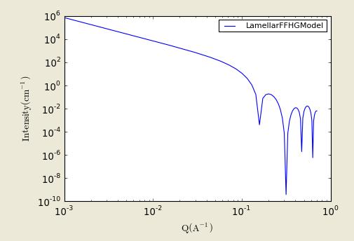
Figure. 1D plot using the default values (w/1000 data point).

Our model uses the form factor calculations implemented in a c-library provided by the NIST Center for Neutron Research (Kline, 2006):

REFERENCE

Nallet, Laversanne, and Roux, J. Phys. II France, 3, (1993) 487-502.

also in J. Phys. Chem. B, 105, (2001) 11081-11088.

2.27. LamellarPSModel

This model provides the scattering intensity (form factor * structure factor), I(q), for a lyotropic lamellar phase where a random distribution in solution are assumed.

The scattering intensity I(q) is:

The form factor is

and the structure is

where

Here d= (repeat) spacing, d = bilayer thickness, the contrast Dr = SLD (headgroup) - SLD(solvent), K=smectic bending elasticity, B=compression modulus, and N = number of lamellar plates (n_plates).

Note: When the Caille parameter is greater than approximately 0.8 to 1.0, the assumptions of the model are incorrect. And due to the complication of the model function, users are responsible to make sure that all the assumptions are handled accurately: see the original reference (below) for more details.

The 2D scattering intensity is calculated in the same way as 1D, where the q vector is defined as.

The returned value is in units of [cm^-1], on absolute scale.

Parameter name	Units	Default value
background	cm^-1	0.0
contrast	Å^-2	5e-006
scale		1
delta	Å	30
n_plates		20
spacing	Å	400
caille	Å^-2	0.1

Figure. 1D plot using the default values (w/6000 data point).

Our model uses the form factor calculations implemented in a c-library provided by the NIST Center for Neutron Research (Kline, 2006):

REFERENCE

Nallet, Laversanne, and Roux, J. Phys. II France, 3, (1993) 487-502.

also in J. Phys. Chem. B, 105, (2001) 11081-11088.

2.28. LamellarPSHGModel

This model provides the scattering intensity (form factor * structure factor), I(q), for a lyotropic lamellar phase where a random distribution in solution are assumed. The SLD of the head region is taken to be different from the SLD of the tail region.

The scattering intensity I(q) is:

The form factor is,

The structure factor is

where

where d_T = tail length (or t_length), d_H = heasd thickness (or h_thickness) , Dr_H = SLD (headgroup) - SLD(solvent), and Dr_T = SLD (tail) - SLD(headgroup). Here d= (repeat) spacing, K=smectic bending elasticity, B=compression modulus, and N = number of lamellar plates (n_plates).

The 2D scattering intensity is calculated in the same way as 1D, where the q vector is defined as.

The returned value is in units of [cm^-1], on absolute scale. In the parameters, sld_tail = SLD of the tail group, sld_head = SLD of the head group, and sld_solvent = SLD of the solvent.

Parameter name	Units	Default value
background	cm^-1	0.001
sld_head	Å^-2	2e-006
scale		1
sld_solvent	Å^-2	6e-006
deltaH	Å	2
deltaT	Å	10
sld_tail	Å^-2	0
n_plates		30
spacing	Å	40
caille	Å^-2	0.001

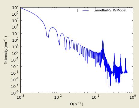
Figure. 1D plot using the default values (w/6000 data point).

Our model uses the form factor calculations implemented in a c-library provided by the NIST Center for Neutron Research (Kline, 2006):

REFERENCE

Nallet, Laversanne, and Roux, J. Phys. II France, 3, (1993) 487-502.

also in J. Phys. Chem. B, 105, (2001) 11081-11088.

2.29. LamellarPCrystalModel

Lamella ParaCrystal Model: Calculates the scattering from a stack of repeating lamellar structures. The stacks of lamellae (infinite in lateral dimension) are treated as a paracrystal to account for the repeating spacing. The repeat distance is further characterized by a Gaussian polydispersity. This model can be used for large multilamellar vesicles.

The scattering intensity I(q) is calculated as:

The form factor of the bilayer is approximated as the cross section of an infinite, planar bilayer of thickness t.

Here, the scale factor is used instead of the mass per area of the bilayer (G). The scale factor is the volume fraction of the material in the bilayer, not the total excluded volume of the paracrystal. ZN(q) describes the interference effects for aggregates consisting of more than one bilayer. The equations used are (3-5) from the Bergstrom reference below.

Non-integer numbers of stacks are calculated as a linear combination of the lower and higher values:

The 2D scattering intensity is the same as 1D, regardless of the orientation of the q vector which is defined as.

The parameters of the model are the following (Nlayers= no. of layers, pd_spacing= polydispersity of spacing…):

Parameter name	Units	Default value
background	cm^-1	0
scale		1
Nlayers		20
pd_spacing		0.2
sld_layer	Å^-2	1e-6
sld_solvent	Å^-2	6.34e-6
spacing	Å	250
thickness	Å	33

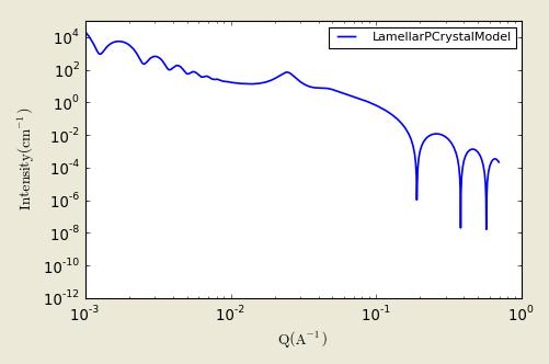
Figure. 1D plot using the default values above (w/20000 data point).

Our model uses the form factor calculations implemented in a c-library provided by the NIST Center for Neutron Research (Kline, 2006).

See the reference for details.

REFERENCE

M. Bergstrom, J. S. Pedersen, P. Schurtenberger, S. U. Egelhaaf, J. Phys. Chem. B, 103 (1999) 9888-9897.

2.30. SC(Simple Cubic Para-)CrystalModel

Calculates the scattering from a simple cubic lattice with paracrystalline distortion. Thermal vibrations are considered to be negligible, and the size of the paracrystal is infinitely large. Paracrystalline distortion is assumed to be isotropic and characterized by a Gaussian distribution.

The returned value is scaled to units of [cm-1sr-1], absolute scale.

The scattering intensity I(q) is calculated as:

where scale is the volume fraction of spheres, Vp is the volume of the primary particle, V(lattice) is a volume correction for the crystal structure, P(q) is the form factor of the sphere (normalized) and Z(q) is the paracrystalline structure factor for a simple cubic structure. Equation (16) of the 1987 reference is used to calculate Z(q), using equations (13)-(15) from the 1987 paper for Z1, Z2, and Z3.

The lattice correction (the occupied volume of the lattice) for a simple cubic structure of particles of radius R and nearest neighbor separation D is:

The distortion factor (one standard deviation) of the paracrystal is included in the calculation of Z(q):

where g is a fractional distortion based on the nearest neighbor distance.

The simple cubic lattice is:

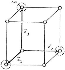
For a crystal, diffraction peaks appear at reduced q-values givn by:

where for a simple cubic lattice any h, k, l are allowed and none are forbidden. Thus the peak positions correspond to (just the first 5):

NOTE: The calculation of Z(q) is a double numerical integral that must be carried out with a high density of points to properly capture the sharp peaks of the paracrystalline scattering. So be warned that the calculation is SLOW. Go get some coffee. Fitting of any experimental data must be resolution smeared for any meaningful fit. This makes a triple integral. Very, very slow. Go get lunch.

REFERENCES

Hideki Matsuoka et. al. Physical Review B, 36 (1987) 1754-1765. (Original Paper)

Hideki Matsuoka et. al. Physical Review B, 41 (1990) 3854 -3856. (Corrections to FCC and BCC lattice structure calculation)

Parameter name	Units	Default value
background	cm^-1	0
dnn	Å	220
scale		1
sldSolv	Å^-2	6.3e-006
radius	Å	40
sld_Sph	Å^-2	3e-006
d_factor		0.06

TEST DATASET

This example dataset is produced using 200 data points, qmin = 0.01 Å-1, qmax = 0.1 Å-1 and the above default values.

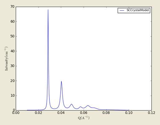
Figure. 1D plot in the linear scale using the default values (w/200 data point).

The 2D (Anisotropic model) is based on the reference (above) which I(q) is approximated for 1d scattering. Thus the scattering pattern for 2D may not be accurate. Note that we are not responsible for any incorrectness of the 2D model computation.

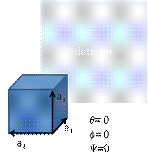
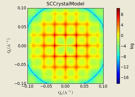
Figure. 2D plot using the default values (w/200X200 pixels).

2.31. FC(Face Centered Cubic Para-)CrystalModel

Calculates the scattering from a face-centered cubic lattice with paracrystalline distortion. Thermal vibrations are considered to be negligible, and the size of the paracrystal is infinitely large. Paracrystalline distortion is assumed to be isotropic and characterized by a Gaussian distribution.

The returned value is scaled to units of [cm-1sr-1], absolute scale.

The scattering intensity I(q) is calculated as:

where scale is the volume fraction of spheres, Vp is the volume of the primary particle, V(lattice) is a volume correction for the crystal structure, P(q) is the form factor of the sphere (normalized) and Z(q) is the paracrystalline structure factor for a face-centered cubic structure. Equation (1) of the 1990 reference is used to calculate Z(q), using equations (23)-(25) from the 1987 paper for Z1, Z2, and Z3.

The lattice correction (the occupied volume of the lattice) for a face-centered cubic structure of particles of radius R and nearest neighbor separation D is:

The distortion factor (one standard deviation) of the paracrystal is included in the calculation of Z(q):

where g is a fractional distortion based on the nearest neighbor distance.

The face-centered cubic lattice is:

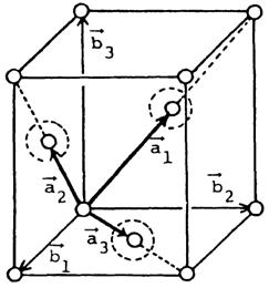
For a crystal, diffraction peaks appear at reduced q-values givn by:

where for a face-centered cubic lattice h, k, l all odd or all even are allowed and reflections where h, k, l are mixed odd/even are forbidden. Thus the peak positions correspond to (just the first 5):

REFERENCES

Hideki Matsuoka et. al. Physical Review B, 36 (1987) 1754-1765. (Original Paper)

Hideki Matsuoka et. al. Physical Review B, 41 (1990) 3854 -3856. (Corrections to FCC and BCC lattice structure calculation)

Parameter name	Units	Default value
background	cm^-1	0
dnn	Å	220
scale		1
sldSolv	Å^-2	6.3e-006
radius	Å	40
sld_Sph	Å^-2	3e-006
d_factor		0.06

TEST DATASET

This example dataset is produced using 200 data points, qmin = 0.01 Å-1, qmax = 0.1 Å-1 and the above default values.

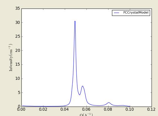
Figure. 1D plot in the linear scale using the default values (w/200 data point).

The 2D (Anisotropic model) is based on the reference (above) in which I(q) is approximated for 1d scattering. Thus the scattering pattern for 2D may not be accurate. Note that we are not responsible for any incorrectness of the 2D model computation.

Figure. 2D plot using the default values (w/200X200 pixels).

2.32. BC(Body Centered Cubic Para-)CrystalModel

Calculates the scattering from a body-centered cubic lattice with paracrystalline distortion. Thermal vibrations are considered to be negligible, and the size of the paracrystal is infinitely large. Paracrystalline distortion is assumed to be isotropic and characterized by a Gaussian distribution.The returned value is scaled to units of [cm-1sr-1], absolute scale.

The scattering intensity I(q) is calculated as:

where scale is the volume fraction of spheres, Vp is the volume of the primary particle, V(lattice) is a volume correction for the crystal structure, P(q) is the form factor of the sphere (normalized) and Z(q) is the paracrystalline structure factor for a body-centered cubic structure. Equation (1) of the 1990 reference is used to calculate Z(q), using equations (29)-(31) from the 1987 paper for Z1, Z2, and Z3.

The lattice correction (the occupied volume of the lattice) for a body-centered cubic structure of particles of radius R and nearest neighbor separation D is:

The distortion factor (one standard deviation) of the paracrystal is included in the calculation of Z(q):

where g is a fractional distortion based on the nearest neighbor distance.

The body-centered cubic lattice is:

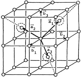
For a crystal, diffraction peaks appear at reduced q-values givn by:

where for a body-centered cubic lattice, only reflections where (h+k+l) = even are allowed and reflections where (h+k+l) = odd are forbidden. Thus the peak positions correspond to (just the first 5):

REFERENCES

Hideki Matsuoka et. al. Physical Review B, 36 (1987) 1754-1765. (Original Paper)

Hideki Matsuoka et. al. Physical Review B, 41 (1990) 3854 -3856. (Corrections to FCC and BCC lattice structure calculation)

Parameter name	Units	Default value
background	cm^-1	0
dnn	Å	220
scale		1
sldSolv	Å^-2	6.3e-006
radius	Å	40
sld_Sph	Å^-2	3e-006
d_factor		0.06

TEST DATASET

This example dataset is produced using 200 data points, qmin = 0.001 Å-1, qmax = 0.1 Å-1 and the above default values.

Figure. 1D plot in the linear scale using the default values (w/200 data point).

The 2D (Anisotropic model) is based on the reference (1987) in which I(q) is approximated for 1d scattering. Thus the scattering pattern for 2D may not be accurate. Note that we are not responsible for any incorrectness of the 2D model computation.

Figure. 2D plot using the default values (w/200X200 pixels).

3. Shape-Independent Models

The following are models used for shape-independent SANS analysis.

3.1. Debye (Model)

The Debye model is a form factor for a linear polymer chain. In addition to the radius of gyration, Rg, a scale factor "scale", and a constant background term are included in the calculation.

For 2D plot, the wave transfer is defined as.

Parameter name	Units	Default value
scale	None	1.0
rg	Å	50.0
background	cm^-1	0.0

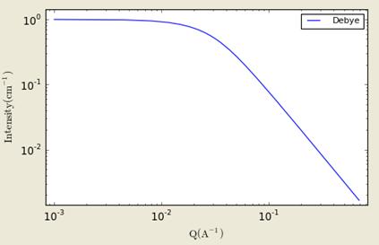
Figure. 1D plot using the default values (w/200 data point).

Reference: Roe, R.-J., "Methods of X-Ray and Neutron Scattering in Polymer Science", Oxford University Press, New York (2000).

3.2. BroadPeak (Model)

Calculate an empirical functional form for SANS data characterized by a broad scattering peak. Many SANS spectra are characterized by a broad peak even though they are from amorphous soft materials. The d-spacing corresponding to the broad peak is a characteristic distance between the scattering inhomogeneities (such as in lamellar, cylindrical, or spherical morphologies or for bicontinuous structures).

The returned value is scaled to units of [cm-1sr-1], absolute scale.

The scattering intensity I(q) is calculated by:

Here the peak position is related to the d-spacing as Q0 = 2pi/d0. Soft systems that show a SANS peak include copolymers, polyelectrolytes, multiphase systems, layered structures, etc.

For 2D plot, the wave transfer is defined as.

Parameter name	Units	Default value
scale_l (= C)		10
scale_p (=A)		1e-05
length_l (=x)	Å	50
q_peak (= Q0)	Å^-1	0.1
exponent_l (=n)		2
exponent_p (=m)		3
Background (=B)	cm^-1	0.1

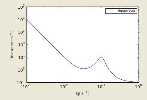
Figure. 1D plot using the default values (w/200 data point).

Reference: None.

3.3. CorrLength (CorrelationLengthModel)

Calculate an empirical functional form for SANS data characterized by a low-Q signal and a high-Q signal

The returned value is scaled to units of [cm-1sr-1], absolute scale.

The scattering intensity I(q) is calculated by:

The first term describes Porod scattering from clusters (exponent = n) and the second term is a Lorentzian function describing scattering from polymer chains (exponent = m). This second term characterizes the polymer/solvent interactions and therefore the thermodynamics. The two multiplicative factors A and C, the incoherent background B and the two exponents n and m are used as fitting parameters. The final parameter (xi) is a correlation length for the polymer chains. Note that when m = 2, this functional form becomes the familiar Lorentzian function.

For 2D plot, the wave transfer is defined as.

Parameter name	Units	Default value
scale_l (= C)		10
scale_p (=A)		1e-06
length_l (=x)	Å	50
exponent_l (=n)		2
exponent_p (=m)		3
Background (=B)	cm^-1	0.1

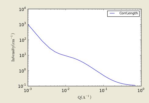
Figure. 1D plot using the default values (w/500 data points).

REFERENCE

B. Hammouda, D.L. Ho and S.R. Kline, “Insight into Clustering in Poly(ethylene oxide) Solutions”, Macromolecules 37, 6932-6937 (2004).

3.4. (Ornstein-Zernicke) Lorentz (Model)

The Ornstein-Zernicke model is defined by:

The parameter L is referred to as the screening length.

For 2D plot, the wave transfer is defined as.

Parameter name	Units	Default value
scale	None	1.0
length	Å	50.0
background	cm^-1	0.0

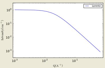
Figure. 1D plot using the default values (w/200 data point).

3.5. DAB (Debye-Anderson-Brumberger)_Model

Calculates the scattering from a randomly distributed, two-phase system based on the Debye-Anderson-Brumberger (DAB) model for such systems. The two-phase system is characterized by a single length scale, the correlation length, which is a measure of the average spacing between regions of phase 1 and phase 2. The model also assumes smooth interfaces between the phases and hence exhibits Porod behavior (I ~ Q^-4) at large Q (Q*correlation length >> 1).

The parameter L is referred to as the correlation length.

For 2D plot, the wave transfer is defined as.

Parameter name	Units	Default value
scale	None	1.0
length	Å	50.0
background	cm^-1	0.0

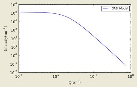
Figure. 1D plot using the default values (w/200 data point).

References:

Debye, Anderson, Brumberger, "Scattering by an Inhomogeneous Solid. II. The Correlation Function and its Application", J. Appl. Phys. 28 (6), 679 (1957).

Debye, Bueche, "Scattering by an Inhomogeneous Solid", J. Appl. Phys. 20, 518 (1949).

3.6. Absolute Power_Law

This model describes a power law with background.

Note the minus sign in front of the exponent.

Parameter name	Units	Default value
Scale	None	1.0
m	None	4
Background	cm^-1	0.0

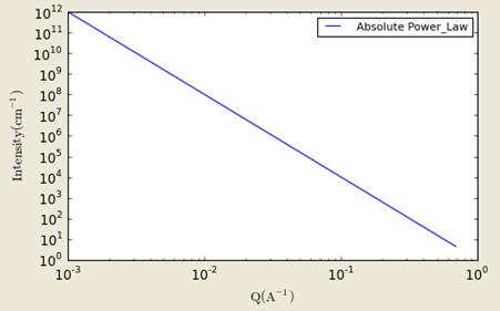
Figure. 1D plot using the default values (w/200 data point).

3.7. Teubner Strey (Model)

This function calculates the scattered intensity of a two-component system using the Teubner-Strey model.

For 2D plot, the wave transfer is defined as.

Parameter name	Units	Default value
scale	None	0.1
c1	None	-30.0
c2	None	5000.0
background	cm^-1	0.0

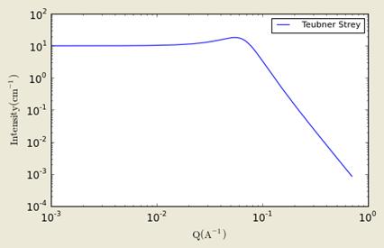
Figure. 1D plot using the default values (w/200 data point).

References:

Teubner, M; Strey, R. J. Chem. Phys., 87, 3195 (1987).

Schubert, K-V., Strey, R., Kline, S. R. and E. W. Kaler, J. Chem. Phys., 101, 5343 (1994).

3.8. FractalModel

Calculates the scattering from fractal-like aggregates built from spherical building blocks following the Texiera reference. The value returned is in cm^-1.

The scale parameter is the volume fraction of the building blocks, R₀ is the radius of the building block, D_f is the fractal dimension, ξ is the correlation length, ρ_solvent is the scattering length density of the solvent, and ρ_block is the scattering length density of the building blocks.

The polydispersion in radius is provided.

For 2D plot, the wave transfer is defined as.

Parameter name	Units	Default value
scale	None	0.05
radius	Å	5.0
fractal_dim	None	2
corr_length	Å	100.0
block_sld	Å^-2	2e-6
solvent_sld	Å^-2	6e-6
background	cm^-1	0.0

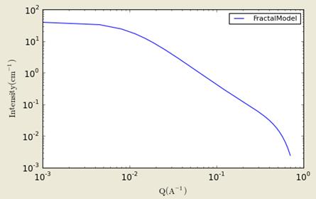
Figure. 1D plot using the default values (w/200 data point).

References:

J. Teixeira, (1988) J. Appl. Cryst., vol. 21, p781-785

3.9. FractalCoreShell(Model)

Calculates the scattering from a fractal structure with a primary building block of core-shell spheres. The fractal structure is as documented in the fractal model. This model could find use for aggregates of coated particles, or aggregates of vesicles. The polydispersity computation of radius and thickness is provided.

The returned value is scaled to units of [cm-1sr-1], absolute scale.

See each of these individual models for full documentation.

For 2D plot, the wave transfer is defined as.

Parameter name	Units	Default value
volfraction		0.05
frac_dim		2
radius	Å	5.0
fractal_dim		2
cor_length	Å	100.0
core_sld	Å^-2	3.5e-6
shell_sld	Å^-2	1e-6
solvent_sld	Å^-2	6.35e-6
background	cm^-1	0.0

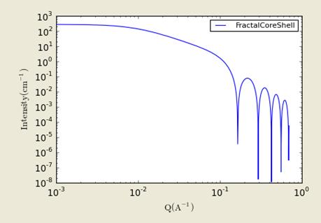
Figure. 1D plot using the default values (w/500 data points).

References:

See the PolyCore and Fractal documentation.

3.10. GaussLorentzGel(Model)

Calculates the scattering from a gel structure, typically a physical network. It is modeled as a sum of a low-q exponential decay plus a lorentzian at higher q-values. It is generally applicable to gel structures.

The returned value is scaled to units of [cm-1sr-1], absolute scale.

The scattering intensity I(q) is calculated as (eqn 5 from the reference):

Uppercase Zeta is the static correlations in the gel, which can be attributed to the "frozen-in" crosslinks of some gels. Lowercase zeta is the dynamic correlation length, which can be attributed to the fluctuating polymer chain between crosslinks. IG(0) and IL(0) are the scaling factors for each of these structures. Your physical system may be different, so think about the interpretation of these parameters.

Note that the peaked structure at higher q values (from Figure 2 of the reference below) is not reproduced by the model. Peaks can be introduced into the model by summing this model with the PeakGauss Model function.

For 2D plot, the wave transfer is defined as.

Parameter name	Units	Default value
dyn_colength(=Dynamic correlation length)	Å	20.0
scale_g(=Gauss scale factor)		100
scale_l(=Lorentzian scale factor)		50
stat_colength(=Static correlation Z)	Å	100.0
background	cm^-1	0.0

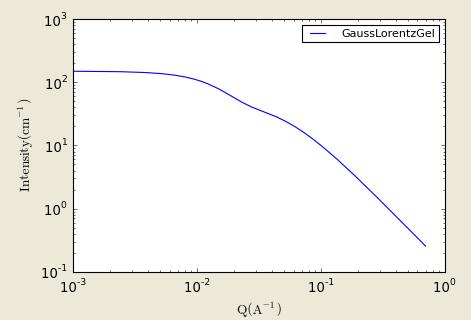
Figure. 1D plot using the default values (w/500 data points).

REFERENCE:

G. Evmenenko, E. Theunissen, K. Mortensen, H. Reynaers, Polymer 42 (2001) 2907-2913.

3.11. BEPolyelectrolyte Model

Calculates the structure factor of a polyelectrolyte solution with the RPA expression derived by Borue and Erukhimovich. The value returned is in cm^-1.

K is a contrast factor of the polymer, L_b is the Bjerrum length, h is the virial parameter, b is the monomer length, C_s is the concentration of monovalent salt, α is the ionization degree, C_a is the polymer molar concentration, and background is the incoherent background.

For 2D plot, the wave transfer is defined as.

Parameter name	Units	Default value
K	Barns = 10^-24 cm²	10
L_b	Å	7.1
h	Å^-3	12
b	Å	10
Cs	Mol/L	0
alpha	None	0.05
Ca	Mol/L	0.7
background	cm^-1	0.0

References:

Borue, V. Y., Erukhimovich, I. Y. Macromolecules 21, 3240 (1988).

Joanny, J.-F., Leibler, L. Journal de Physique 51, 545 (1990).

Moussaid, A., Schosseler, F., Munch, J.-P., Candau, S. J. Journal de Physique II France

3, 573 (1993).

Raphaël, E., Joanny, J.-F., Europhysics Letters 11, 179 (1990).

3.12. Guinier (Model)

A Guinier analysis is done by linearizing the data at low q by plotting it as log(I) versus Q². The Guinier radius R_g can be obtained by fitting the following model:

For 2D plot, the wave transfer is defined as.

Parameter name	Units	Default value
scale	cm^-1	1.0
Rg	Å	0.1

3.13. GuinierPorod (Model)

Calculates the scattering for a generalized Guinier/power law object. This is an empirical model that can be used to determine the size and dimensionality of scattering objects.

The returned value is P(Q) as written in equation (1), plus the incoherent background term. The result is in the units of [cm-1sr-1], absolute scale.

A Guinier-Porod empirical model can be used to fit SAS data from asymmetric objects such as rods or platelets. It also applies to intermediate shapes between spheres and rod or between rods and platelets. The following functional form is used:

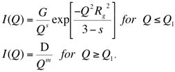(1)

This is based on the generalized Guinier law for such elongated objects [2]. For 3D globular objects (such as spheres), s = 0 and one recovers the standard Guinier formula. For 2D symmetry (such as for rods) s = 1 and for 1D symmetry (such as for lamellae or platelets) s = 2. A dimensionality parameter 3-s is defined, and is 3 for spherical objects, 2 for rods, and 1 for plates.

Enforcing the continuity of the Guinier and Porod functions and their derivatives yields:

and

Note that the radius of gyration for a sphere of radius R is given by R_g = R sqrt(3/5) ,

that for the cross section of an randomly oriented cylinder of radius R is given by R_g = R / sqrt(2).

The cross section of a randomly oriented lamella of thickness T is given by R_g = T / sqrt(12).

The intensity given by Eq. 1 is the calculated result, and is plotted below for the default parameter values.

REFERENCE

[1] Guinier, A.; Fournet, G. "Small-Angle Scattering of X-Rays", John Wiley and Sons, New York, (1955).

[2] Glatter, O.; Kratky, O., “Small-Angle X-Ray Scattering”, Academic Press (1982). Check out Chapter 4 on Data Treatment, pages 155-156.

For 2D plot, the wave transfer is defined as.

Parameter name	Units	Default value
Scale(=Guinier scale, G)	cm^-1	1.0
rg	Å	100
dim(=Dimensional Variable, s)		1
m(=Porod exponent)		3
background		0.1

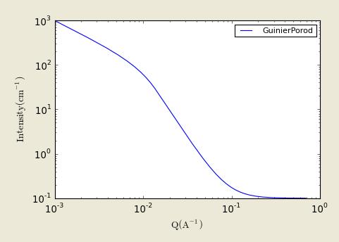
Figure. 1D plot using the default values (w/500 data points).

3.14. PorodModel

A Porod analysis is done by linearizing the data at high q by plotting it as log(I) versus log(Q). In the high q region we can fit the following model:

C is the scale factor and Sv is the specific surface area of the sample and Δρ is the contrast factor.

The background term is added for data analysis.

For 2D plot, the wave transfer is defined as.

Parameter name	Units	Default value
scale	Å^-4	0.1
background	cm^-1	0

3.15. PeakGaussModel

Model describes a Gaussian shaped peak including a flat background,

with the peak having height of I0 centered at qpk having standard deviation of B. The fwhm is 2.354*B.

Parameters I0, B, qpk, and BGD can all be adjusted during fitting.

REFERENCE: None

For 2D plot, the wave transfer is defined as.

Parameter name	Units	Default value
scale	cm^-1	100
q0	Å	0.05
B		0.005
background		1

Figure. 1D plot using the default values (w/500 data points).

3.16. PeakLorentzModel

Model describes a Lorentzian shaped peak including a flat background,

with the peak having height of I0 centered at qpk having a hwhm (half-width-half-maximum) of B.

The parameters I0, B, qpk, and BGD can all be adjusted during fitting.

REFERENCE: None

For 2D plot, the wave transfer is defined as.

Parameter name	Units	Default value
scale	cm^-1	100
q0	Å	0.05
B		0.005
background		1

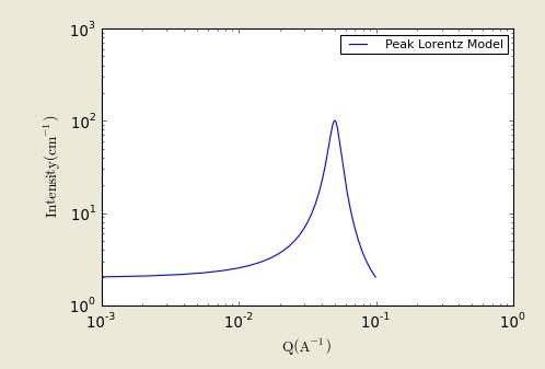
Figure. 1D plot using the default values (w/500 data points).

3.17. Poly_GaussCoil (Model)

Polydisperse Gaussian Coil: Calculate an empirical functional form for scattering from a polydisperse polymer chain ina good solvent. The polymer is polydisperse with a Schulz-Zimm polydispersity of the molecular weight distribution.

The returned value is scaled to units of [cm-1sr-1], absolute scale.

where the dimensionless chain dimension is:

and the polydispersion is

The scattering intensity I(q) is calculated as:

The polydispersion in ‘rg’ is provided.

For 2D plot, the wave transfer is defined as.

TEST DATASET

This example dataset is produced by running the Poly_GaussCoil, using 200 data points, qmin = 0.001 Å-1, qmax = 0.7 Å-1 and the default values below.

Parameter name	Units	Default value
Scale	None	1.0
rg	Å	60.0
poly_m	Mw/Mn	2
background	cm^-1	0.001

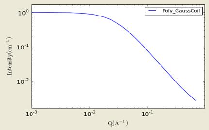
Figure. 1D plot using the default values (w/200 data point).

Reference:

Glatter & Kratky - pg.404.

J.S. Higgins, and H.C. Benoit, “Polymers and Neutron Scattering”, Oxford Science

Publications (1996).

3.18. PolymerExclVolume (Model)

Calculates the scattering from polymers with excluded volume effects.

The returned value is scaled to units of [cm-1sr-1], absolute scale.

The returned value is P(Q) as written in equation (2), plus the incoherent background term. The result is in the units of [cm-1sr-1], absolute scale.

A model describing polymer chain conformations with excluded volume was introduced to describe the conformation of polymer chains, and has been used as a template for describing mass fractals. The form factor for that model (Benoit, 1957) was originally presented in the following integral form:

(1)

Here n is the excluded volume parameter which is related to the Porod exponent m as n = 1/m, a is the polymer chain statistical segment length and n is the degree of polymerization. This integral was later put into an “almost” analytical form (Hammouda, 1993) as follows:

(2)

Here, g(x,U) is the incomplete gamma function which is a built-in function in computer libraries.

The variable U is given in terms of the scattering variable Q as:

The radius of gyration squared has been defined as:

Note that this model describing polymer chains with excluded volume applies only in the mass fractal range ( 5/3 <= m <= 3) and does not apply to surface fractals ( 3 < m <= 4). It does not reproduce the rigid rod limit (m = 1) because it assumes chain flexibility from the outset. It may cover a portion of the semiflexible chain range ( 1 < m < 5/3).

The low-Q expansion yields the Guinier form and the high-Q expansion yields the Porod form which is given by:

Here G(x) = g(x,inf) is the gamma function. The asymptotic limit is dominated by the first term:

The special case when n = 0.5 (or m = 1/n = 2) corresponds to Gaussian chains for which the form factor is given by the familiar Debye function.

The form factor given by Eq. 2 is the calculated result, and is plotted below for the default parameter values.

REFERENCE

Benoit, H., Comptes Rendus (1957). 245, 2244-2247.

Hammouda, B., “SANS from Homogeneous Polymer Mixtures A Unified Overview”, Advances in Polym. Sci. (1993), 106, 87-133.

For 2D plot, the wave transfer is defined as.

TEST DATASET

This example dataset is produced, using 200 data points, qmin = 0.001 Å-1, qmax = 0.2 Å-1 and the default values below.

Parameter name	Units	Default value
Scale	None	1.0
rg	Å	60.0
m(=Porod exponent)		3
background	cm^-1	0.0

Figure. 1D plot using the default values (w/500 data points).

3.19. RPA10Model

Calculates the macroscopic scattering intensity (units of cm^-1) for a multicomponent homogeneous mixture of polymers using the Random Phase Approximation. This general formalism contains 10 specific cases:

Case 0: C/D Binary mixture of homopolymers

Case 1: C-D Diblock copolymer

Case 2: B/C/D Ternary mixture of homopolymers

Case 3: C/C-D Mixture of a homopolymer B and a diblock copolymer C-D

Case 4: B-C-D Triblock copolymer

Case 5: A/B/C/D Quaternary mixture of homopolymers

Case 6: A/B/C-D Mixture of two homopolymers A/B and a diblock C-D

Case 7: A/B-C-D Mixture of a homopolymer A and a triblock B-C-D

Case 8: A-B/C-D Mixture of two diblock copolymers A-B and C-D

Case 9: A-B-C-D Four-block copolymer

Note: the case numbers are different from the IGOR/NIST SANS package.

Only one case can be used at any one time. Plotting a different case will overwrite the original parameter waves.

The returned value is scaled to units of [cm-1].

Component D is assumed to be the "background" component (all contrasts are calculated with respect to component D).

Scattering contrast for a C/D blend= {SLD (component C) - SLD (component D)}2

Depending on what case is used, the number of fitting parameters varies. These represent the segment lengths (ba, bb, etc) and the Chi parameters (Kab, Kac, etc). The last one of these is a scaling factor to be held constant equal to unity.

The input parameters are the degree of polymerization, the volume fractions for each component the specific volumes and the neutron scattering length densities.

This RPA (mean field) formalism applies only when the multicomponent polymer mixture is in the homogeneous mixed-phase region.

REFERENCE

A.Z. Akcasu, R. Klein and B. Hammouda, Macromolecules 26, 4136 (1993)

Fitting parameters for Case0 Model

Parameter name	Units	Default value
background	cm^-1	0.0
scale		1
bc(=Seg. Length bc)		5
bd(=Seg. Length bd)		5
Kcd(Chi Param. Kcd)		-0.0004

Fixed parameters for Case0 Model

Parameter name	Units	Default value
Lc(= Scatter. Length_c)		1e-12
Ld(= Scatter. Length_d)		0
Nc(=Deg.Polym.c)		1000
Nd(=Deg.Polym.d)		1000
Phic(=Vol. fraction of c)		0.25
Phid(=Vol. fraction of d)		0.25
vc(=Spec. vol. of c)		100
vd(=Spec. vol. of d)		100

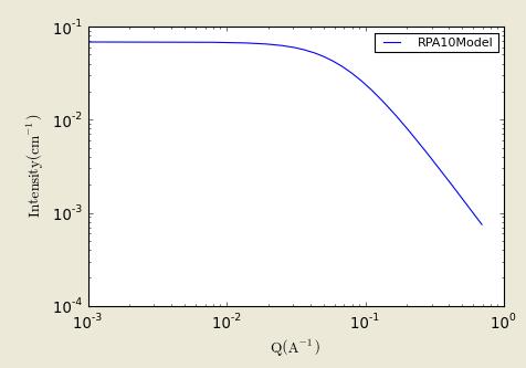
Figure. 1D plot using the default values (w/500 data points).

3.20. TwoLorentzian(Model)

Calculate an empirical functional form for SANS data characterized by a two Lorentzian functions.

The returned value is scaled to units of [cm-1sr-1], absolute scale.

The scattering intensity I(q) is calculated by:

A = Lorentzian scale #1

C = Lorentzian scale #2

where ‘scale’ is the peak height centered at q₀, and B refers to the standard deviation of the function.

The background term is added for data analysis.

For 2D plot, the wave transfer is defined as.

Default input parameter values

Parameter name	Units	Default value
scale_1(=A)		10
scale_2(=C)		1
1ength_1 (=Correlation length1)	Å	100
1ength_2(=Correlation length2)	Å	10
exponent_1(=n)		3
exponent_2(=m)		2
Background(=B)	cm^-1	0.1

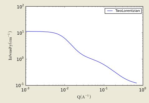
Figure. 1D plot using the default values (w/500 data points).

REFERENCE: None

3.21. TwoPowerLaw(Model)

Calculate an empirical functional form for SANS data characterized by two power laws.

The returned value is scaled to units of [cm-1sr-1], absolute scale.

The scattering intensity I(q) is calculated by:

qc is the location of the crossover from one slope to the other. The scaling A, sets the overall intensity of the lower Q power law region. The scaling of the second power law region is scaled to match the first. Be sure to enter the power law exponents as positive values.

For 2D plot, the wave transfer is defined as.

Default input parameter values

Parameter name	Units	Default value
coef_A		1.0
qc	Å^-1	0.04
power_1(=m1)		4
power_2(=m2)		4
background	cm^-1	0.0

Figure. 1D plot using the default values (w/500 data points).

3.22. UnifiedPower(Law and)Rg(Model)

The returned value is scaled to units of [cm-1sr-1], absolute scale.

Note that the level 0 is an extra function that is the inverse function; I (q) = scale/q + background.

Otherwise, program incorporates the empirical multiple level unified Exponential/Power-law fit method developed by G. Beaucage. Four functions are included so that One, Two, Three, or Four levels can be used.

The empirical expressions are able to reasonably approximate the scattering from many different types of particles, including fractal clusters, random coils (Debye equation), ellipsoidal particles, etc. The empirical fit function is

For each level, the four parameters Gi, Rg,i, Bi and Pi must be chosen.

For example, to approximate the scattering from random coils (Debye equation), set Rg,i as the Guinier radius, Pi = 2, and Bi = 2 Gi / Rg,i

See the listed references for further information on choosing the parameters.

For 2D plot, the wave transfer is defined as.

Default input parameter values

Parameter name	Units	Default value
scale		1.0
Rg2	Å	21
power2		2
G2	cm^-1sr^-1	3
B2	cm^-1sr^-1	0.0006
Rg1	Å	15.8
power1		4
G1	cm^-1sr^-1	400
B1	cm^-1sr^-1	4.5e-006
background	cm^-1	0.0

Figure. 1D plot using the default values (w/500 data points).

REFERENCES

G. Beaucage (1995). J. Appl. Cryst., vol. 28, p717-728.

G. Beaucage (1996). J. Appl. Cryst., vol. 29, p134-146.

3.23. LineModel

This is a linear function that calculates:

where A and B are the coefficients of the first and second order terms.

Note: For 2D plot, I(q) = I(q_x)*I(q_y) which is defined differently from other shape independent models.

Parameter name	Units	Default value
A	cm^-1	1.0
B	Å	1.0

4. Customized Models

Customized model functions can be redefined or added by users (See SansView tutorial for details).

4.1. A+Bcos(2x)+Csin(2x)

This function, as an example of a user defined function, calculates the intensity = A + Bcos(2q) + Csin(2q).

4.2. sin(poly)/poly

This function, as an example of a user defined function, calculates the intensity = scale * sin(f)/f, where f = A + Bq + Cq² + Dq³+ Eq⁴ + Fq⁵.

4.3. Sum[P1(Cyl), P2(PEV)]

This function, as an example of a user defined function, calculates the intensity = scale_factor * (CylinderModel + PolymerExclVolume model). To make your own sum(P1+P2) model, modify and save the file named 'sum_p1_p2.py' in the SansView/plugins/ folder by changing the model names in the 'from' and 'import' statement, and the self.name if desired. It works only for single functional models.

4.4. ReflectivityModel

This model calculates the reflectivity and uses the Parrett algorithm. Up to nine film layers are supported between Bottom(substrate) and Medium(Superstrate where the neutron enters the first top film). Each layers are composed of [ ½ of the interface(from the previous layer or substrate) + flat portion + ½ of the interface(to the next layer or medium)]. Only two simple interfacial functions are selectable, error function and linear function. The each interfacial thickness is equivalent to (- 2.5 sigma to +2.5 sigma for the error function, sigma=roughness).

Note: This model was contributed by an interested user.

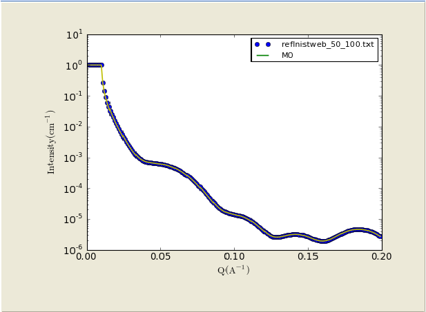
Figure. Comparison (using the SLD profile below) with NISTweb calculation (circles): http://www.ncnr.nist.gov/resources/reflcalc.html.

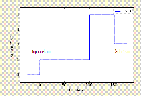
Figure. SLD profile used for the calculation(above).

4.5. ReflectivityIIModel

Same as the ReflectivityModel except that the it is more customizable. More interfacial functions are supplied. The number of points (npts_inter) for each interface can be choosen. The constant (A below but 'nu' as a parameter name of the model) for exp, erf, or power-law is an input. The SLD at the interface between layers, r_{inter_i}, is calculated with a function chosen by a user, where the functions are:

1) Erf;

2) Power-Law;

3) Exp;

Note: This model was implemented by an interested user.

5. Structure Factors

The information in this section is originated from NIST SANS IgorPro package.

5.1. HardSphere Structure

This calculates the interparticle structure factor for monodisperse spherical particles interacting through hard sphere (excluded volume) interactions. The calculation uses the Percus-Yevick closure where the interparticle potential is:

where r is the distance from the center of the sphere of a radius R.

For 2D plot, the wave transfer is defined as.

Parameter name	Units	Default value
effect_radius	Å	50.0
volfraction		0.2

Figure. 1D plot using the default values (in linear scale).

References:

Percus, J. K.; Yevick, J. Phys. Rev. 110, 1. (1958).

5.2. SquareWell Structure

This calculates the interparticle structure factor for a squar well fluid spherical particles The mean spherical approximation (MSA) closure was used for this calculation, and is not the most appropriate closure for an attractive interparticle potential. This solution has been compared to Monte Carlo simulations for a square well fluid, showing this calculation to be limited in applicability to well depths e < 1.5 kT and volume fractions f < 0.08.

Positive well depths correspond to an attractive potential well. Negative well depths correspond to a potential "shoulder", which may or may not be physically reasonable.

The well width (l) is defined as multiples of the particle diameter (2*R)

The interaction potential is:

where r is the distance from the center of the sphere of a radius R.

For 2D plot, the wave transfer is defined as.

Parameter name	Units	Default value
effect_radius	Å	50.0
volfraction		0.04
welldepth	kT	1.5
wellwidth	diameters	1.2

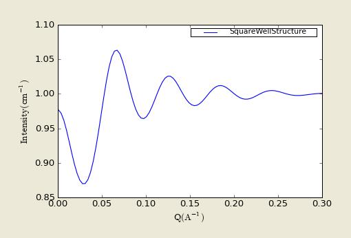
Figure. 1D plot using the default values (in linear scale).

References:

Sharma, R. V.; Sharma, K. C. Physica, 89A, 213. (1977).

5.3. HayterMSA Structure

This calculates the Structure factor (the Fourier transform of the pair correlation function g(r)) for a system of charged, spheroidal objects in a dielectric medium. When combined with an appropriate form factor (such as sphere, core+shell, ellipsoid etc…), this allows for inclusion of the interparticle interference effects due to screened coulomb repulsion between charged particles. This routine only works for charged particles. If the charge is set to zero the routine will self destruct. For non-charged particles use a hard sphere potential.

The salt concentration is used to compute the ionic strength of the solution which in turn is used to compute the Debye screening length. At present there is no provision for entering the ionic strength directly nor for use of any multivalent salts. The counterions are also assumed to be monovalent.

For 2D plot, the wave transfer is defined as.

Parameter name	Units	Default value
effect_radius	Å	20.8
charge		19
volfraction		0.2
temperature	K	318
salt conc	M	0
dielectconst		71.1

Figure. 1D plot using the default values (in linear scale).

References:

JP Hansen and JB Hayter, Molecular Physics 46, 651-656 (1982).

JB Hayter and J Penfold, Molecular Physics 42, 109-118 (1981).

5.4. StickyHS Structure

This calculates the interparticle structure factor for a hard sphere fluid with a narrow attractive well. A perturbative solution of the Percus-Yevick closure is used. The strength of the attractive well is described in terms of "stickiness" as defined below. The returned value is a dimensionless structure factor, S(q).

The perturb (perturbation parameter), epsilon, should be held between 0.01 and 0.1. It is best to hold the perturbation parameter fixed and let the "stickiness" vary to adjust the interaction strength. The stickiness, tau, is defined in the equation below and is a function of both the perturbation parameter and the interaction strength. Tau and epsilon are defined in terms of the hard sphere diameter (sigma = 2R), the width of the square well, delta (same units as R), and the depth of the well, u_o, in units of kT. From the definition, it is clear that smaller tau mean stronger attraction.

where the interaction potential is

The Percus-Yevick (PY) closure was used for this calculation, and is an adequate closure for an attractive interparticle potential. This solution has been compared to Monte Carlo simulations for a square well fluid, with good agreement.

The true particle volume fraction, f, is not equal to h, which appears in most of the reference. The two are related in equation (24) of the reference. The reference also describes the relationship between this perturbation solution and the original sticky hard sphere (or adhesive sphere) model by Baxter.

NOTES: The calculation can go haywire for certain combinations of the input parameters, producing unphysical solutions - in this case errors are reported to the command window and the S(q) is set to -1 (it will disappear on a log-log plot). Use tight bounds to keep the parameters to values that you know are physical (test them) and keep nudging them until the optimization does not hit the constraints.

For 2D plot, the wave transfer is defined as.

Parameter name	Units	Default value
effect_radius	Å	50
perturb		0.05
volfraction		0.1
stickiness	K	0.2

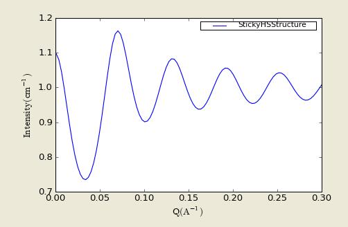
Figure. 1D plot using the default values (in linear scale).

References:

Menon, S. V. G., Manohar, C. and K. Srinivas Rao J. Chem. Phys., 95(12), 9186-9190 (1991).

References

Feigin, L. A, and D. I. Svergun (1987) "Structure Analysis by Small-Angle X-Ray and Neutron Scattering", Plenum Press, New York.

Guinier, A. and G. Fournet (1955) "Small-Angle Scattering of X-Rays", John Wiley and Sons, New York.

Kline, S. R. (2006) J Appl. Cryst. 39(6), 895.

Hansen, S., (1990) J. Appl. Cryst. 23, 344-346.

Henderson, S.J. (1996) Biophys. J. 70, 1618-1627

Stöckel, P., May, R., Strell, I., Cejka, Z., Hoppe, W., Heumann, H., Zillig, W. and Crespi, H. (1980) Eur. J. Biochem. 112, 411-417.

McAlister, B.C. and Grady, B.P., (1998) J. Appl. Cryst. 31, 594-599.

Porod, G. (1982) in Small Angle X-ray Scattering, editors Glatter, O. and Kratky, O., Academic Press.

*Also, see the references at the end of the each model function descriptions.