Model Functions
- Introduction
- Shapes: SphereModel, FuzzySphereModel, CoreShellModel, CoreFourShellModel, VesicleModel, MultiShellModel, BinaryHSModel, CylinderModel, CoreShellCylinderModel, HollowCylinderModel, FlexibleCylinderModel, FlexCylEllipXModel, StackedDisksModel, ParallelepipedModel, EllipticalCylinderModel, EllipsoidModel, CoreShellEllipsoidModel, TriaxialEllipsoidModel, LamellarModel, LamellarFFHGModel, LamellarPSModel, LamellarPSHGModel.
- Shape-Independent: Debye, Lorentz, DAB_Model, Power_Law, Teubner Strey, BEPolyelectrolyte, FractalModel, Guinier, PorodModel, Poly_GaussCoil, Peak Gauss Model, Peak Lorentz Model, LineModel.
- Customized Models: A+Bcos(2x)+Csin(2x), sin(poly)/poly.
- Structure Factors: HardSphereStructure, SquareWellStructure, HayterMSAStructure, StickyHSStructure.
- References
1. Introduction
The present text documents the modules made available by the DANSE software for SANS.
Readers are also referred to the SANS/DANSE wiki page:
http://danse.us/trac/sans
Users can report a bug at the following URL:
http://danse.us/trac/sans/newticket
Note: Our model uses the form factor calculations implemented in a c-library provided by the NIST Center for Neutron Research and thus some content and figures in this document are originated from or shared with the NIST Igor analysis package by permission (S. Kline, NIST, 2006).
2. Shapes (Scattering Intensity Models)
This software provides form factors for various particle shapes. After giving a mathematical definition of each model, we draw the list of parameters available to the user. Validation plots for each model are also presented. Instructions on how to use the software is available with the source code, available from SVN:
svn co svn://danse.us/sans/releases/sansmodels-x.x
To easily compare to the scattering intensity measured in experiments, we normalize the form factors by the volume of the particle:
![]()
with
![]()
where P0(q) is the un-normalized form factor, ρ(r) is the scattering length density at a given point in space and the integration is done over the volume V of the scatterer.
For systems without inter-particle interference, the form
factors we provide can be related to the scattering intensity by the particle
volume fraction:![]() .
.
Our so-called 1D scattering intensity functions provide P(q) for the case where the scatterer is randomly oriented. In that case, the scattering intensity only depends on the length of q. The intensity measured on the plane of the SANS detector will have an azimuthal symmetry around q=0.
Our so-called 2D scattering intensity functions provide P(q, φ) for an oriented system as a function of a q-vector in the plane of the detector. We define the angle φ as the angle between the q vector and the horizontal (x) axis of the plane of the detector.
2.1. Sphere Model
This model provides the form factor, P(q), for a monodisperse spherical particle with uniform scattering length density. The form factor is normalized by the particle volume as described below.
1.1. Definition
The 1D scattering intensity is calculated in the following way (Guinier, 1955):

where scale is a scale factor* volume fraction, V is the volume of the scatterer, r is the radius of the sphere, bkg is the background level and Δρ (contrast) is the scattering length density (SLD) difference between the scatterer and the solvent it is in.
The 2D scattering intensity is the same as P(q) above, regardless of the orientation of the q vector.
The returned value is scaled to units of [cm-1] and the parameters of the sphere model are the following:
|
Parameter name |
Units |
Default value |
|
scale |
None |
1 |
|
radius |
Å |
60 |
|
sldSph |
Å -2 |
2.0e-6 |
|
sldSolv |
Å -2 |
1.0e-6 |
|
background |
cm-1 |
0 |
Our model uses the form factor calculations implemented in a c-library provided by the NIST Center for Neutron Research (Kline, 2006).
2.1. Validation of the sphere model
Validation of our code was done by comparing the output of the 1D model to the output of the software provided by the NIST (Kline, 2006). Figure 1 shows a comparison of the output of our model and the output of the NIST software.

Figure 1: Comparison of the DANSE scattering intensity for a sphere with the output of the NIST SANS analysis software. The parameters were set to: Scale=1.0, Radius=60 Å, Contrast=1e-6 Å -2, and Background=0.01 cm -1.
This model is to calculate the scattering from spherical particles with a "fuzzy" interface.
1.1. Definition
The 1D scattering intensity is calculated in the following way (Guinier, 1955):
The returned value is scaled to units of [cm-1 sr-1], absolute scale.
The scattering intensity I(q) is calculated as:
![]()
![]()
where the amplitude A(q) is given as the typical sphere scattering convoluted with a Gaussian to get a gradual drop-off in the scattering length density:

Here A2(q) is the form factor, P(q). The ‘scale’ is equivalent to the volume fraction of spheres, each of volume, V. Contrast (Δρ ) is the difference of scattering length densities of the sphere and the surrounding solvent.
The poly-dispersion in radius and in fuzziness is provided.
(direct from the reference)
The "fuzziness" of the interface is defined by the parameter (sigma)fuzzy. The particle radius R represents the radius of the particle where the scattering length density profile decreased to 1/2 of the core density. The (sigma)fuzzy is the width of the smeared particle surface: i.e., the standard deviation from the average height of the fuzzy interface. The inner regions [] that display a higher density are described by the radial box profile extending to a radius of approximately Rbox ~ R - 2(sigma). the profile approaches zero as Rsans ~ R + 2(sigma).
For 2D data: The 2D scattering intensity is calculated in
the same way as 1D, where the q vector is defined as![]() .
.
REFERENCE
M. Stieger, J. S. Pedersen, P. Lindner, W. Richtering, Langmuir 20 (2004) 7283-7292.
TEST DATASET
This example dataset is produced by running the FuzzySphereModel, using 200 data points, qmin = 0.001 Å-1, qmax = 0.7 A-1 and the default coef_fuzz values:
|
Parameter name |
Units |
Default value |
|
scale |
None |
1.0 |
|
radius |
Å |
60 |
|
fuzziness |
Å |
10 |
|
sldSolv |
Å -2 |
3e-6 |
|
sldSph |
Å -2 |
1e-6 |
|
background |
cm-1 |
0.001 |

Figure. 1D plot using the default values (w/200 data point).
2.3. Core Shell (Sphere) Model
This model provides the form factor, P(q), for a spherical particle with a core-shell structure. The form factor is normalized by the particle volume.
1.1. Definition
The 1D scattering intensity is calculated in the following way (Guinier, 1955):

where scale is a scale factor, Vs is the volume of the outer shell, Vc is the volume of the core, rs is the radius of the shell, rc is the radius of the core, ρc is the scattering length density of the core, ρs is the scattering length density of the shell, ρsolv is the scattering length density of the solvent, and bkg is the background level.
The 2D scattering intensity is the same as P(q) above, regardless of the orientation of the q vector.
For P*S: The outer most radius (= radius + thickness) is used as the effective radius toward S(Q) when P(Q)*S(Q) is applied.
The returned value is scaled to units of [cm-1] and the parameters of the core-shell sphere model are the following:
Here, radius = the radius of the core and thickness = the thickness of the shell.
|
Parameter name |
Units |
Default value |
|
scale |
None |
1.0 |
|
(core) radius |
Å |
60 |
|
thickness |
Å |
10 |
|
core_sld |
Å -2 |
1e-6 |
|
shell_sld |
Å -2 |
2e-6 |
|
solvent_sld |
Å -2 |
3e-6 |
|
background |
cm-1 |
0.001 |
Our model uses the form factor calculations implemented in a c-library provided by the NIST Center for Neutron Research (Kline, 2006).
REFERENCE
Guinier, A. and G. Fournet, "Small-Angle Scattering of X-Rays", John Wiley and Sons, New York, (1955).
2.1. Validation of the core-shell sphere model
Validation of our code was done by comparing the output of the 1D model to the output of the software provided by the NIST (Kline, 2006). Figure 1 shows a comparison of the output of our model and the output of the NIST software.

Figure 7: Comparison of the DANSE scattering intensity for a core-shell sphere with the output of the NIST SANS analysis software. The parameters were set to: Scale=1.0, Radius=60 Å, Contrast=1e-6 Å -2, and Background=0.001 cm -1.
2.4. CoreFourShell(Sphere)Model
This model provides the scattering from monodisperse core 4 shell structures. It has a core of a specified radius, with four shells. The SLDs of the core and each shell are individually specified.
1.1. Definition
The returned value is scaled to units of [cm-1sr-1], absolute scale.
This model is a trivial extension of the CoreShell function to a larger number of shells. See the CoreShell function for a diagram and documentation.
Be careful that the SLDs and scale can be highly correlated. Hold as many of these fixed as possible.
The 2D scattering intensity is the same as P(q) of 1D, regardless of the orientation of the q vector.
For P*S: The outer most radius (= radius + 4 thicknesses) is used as the effective radius toward S(Q) if P(Q)*S(Q) is applied.
The returned value is scaled to units of [cm-1] and the parameters of the CoreFourshell sphere model are the following:
Here, rad_core = the radius of the core, thick_shelli = the thickness of the shell i and sld_shelli = the SLD of the shell i.
And the sld_core and the sld_solv are the SLD of the core and the solvent, respectively.
|
Parameter name |
Units |
Default value |
|
scale |
None |
1.0 |
|
rad_core |
Å |
60 |
|
sld_core |
Å -2 |
6.4e-6 |
|
sld_shell1 |
Å -2 |
1e-6 |
|
sld_shell2 |
Å -2 |
2e-6 |
|
sld_shell3 |
Å -2 |
3e-6 |
|
sld_shell4 |
Å -2 |
4e-6 |
|
sld_solv |
Å -2 |
6.4e-6 |
|
thick_shell1 |
Å |
10 |
|
thick_shell2 |
Å |
10 |
|
thick_shell3 |
Å |
10 |
|
thick_shell4 |
Å |
10 |
|
background |
cm-1 |
0.001 |
Our model uses the form factor calculations implemented in a c-library provided by the NIST Center for Neutron Research (Kline, 2006).
REFERENCE
See the CoreShell documentation.
TEST DATASET
This example dataset is produced by running the CoreFourShellModel using 200 data points, qmin = 0.001 Å-1, qmax = 0.7 Å-1 and the above default values.

Figure. 1D plot using the default values (w/200 data point).
2.5. VesicleModel
This model provides the form factor, P(q), for an unilamellar vesicle. The form factor is normalized by the volume of the shell.
The 1D scattering intensity is calculated in the following way (Guinier, 1955):

where scale is a scale factor, Vshell is the volume of the shell, V1 is the volume of the core, V2 is the total volume, R1 is the radius of the core, r2 is the outer radius of the shell, ρ1 is the scattering length density of the core and the solvent, ρ2 is the scattering length density of the shell, and bkg is the background level. And J1 = (sinx - xcosx)/x2. The functional form is identical to a "typical" core-shell structure, except that the scattering is normalized by the volume that is contributing to the scattering, namely the volume of the shell alone. Also, the vesicle is best defined in terms of a core radius (= R1) and a shell thickness, t.

The 2D scattering intensity is the same as P(q)
above, regardless of the orientation of the q vector which is
defined as![]() .
.
For P*S: The outer most radius (= radius + thickness) is used as the effective radius toward S(Q) when P(Q)*S(Q) is applied.
The returned value is scaled to units of [cm-1] and the parameters of the vesicle model are the following:
In the parameters, the ‘radius’ represents the core radius (R1) and the ‘thickness’ (R2 – R1) is the shell thickness.
|
Parameter name |
Units |
Default value |
|
scale |
None |
1.0 |
|
radius |
Å |
100 |
|
thickness |
Å |
30 |
|
core_sld |
Å -2 |
6.3e-6 |
|
shell_sld |
Å -2 |
0 |
|
background |
cm-1 |
0.0 |
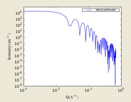
Figure. 1D plot using the default values (w/200 data point).
Our model uses the form factor calculations implemented in a c-library provided by the NIST Center for Neutron Research (Kline, 2006).
REFERENCE
Guinier, A. and G. Fournet, "Small-Angle Scattering of X-Rays", John Wiley and Sons, New York, (1955).
2.6. MultiShellModel
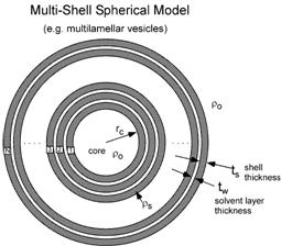
This model provides the form factor, P(q), for a multi-lamellar vesicle with N shells where the core is filled with solvent and the shells are interleaved with layers of solvent. For N = 1, this return to the vesicle model (above).
The 2D scattering intensity is the same as 1D, regardless of
the orientation of the q vector which is defined as![]() .
.
For P*S: The outer most radius (= core_radius + n_pairs * s_thickness + (n_pairs -1) * w_thickness) is used as the effective radius toward S(Q) when P(Q)*S(Q) is applied.
The returned value is scaled to units of [cm-1] and the parameters of the multi-shell model are the following:
In the parameters, the ‘s_thickness’ is the shell thickness while the ‘w_thickness’ is the solvent thickness, and the n_pair is the number of shells.
|
Parameter name |
Units |
Default value |
|
scale |
None |
1.0 |
|
core_radius |
Å |
60.0 |
|
n_pairs |
None |
2.0 |
|
core_sld |
Å -2 |
6.3e-6 |
|
shell_sld |
Å -2 |
0.0 |
|
background |
cm-1 |
0.0 |
|
s_thickness |
Å |
10 |
|
w_thickness |
Å |
10 |

Figure. 1D plot using the default values (w/200 data point).
Our model uses the form factor calculations implemented in a c-library provided by the NIST Center for Neutron Research (Kline, 2006).
REFERENCE
Cabane, B., Small Angle Scattering Methods, Surfactant Solutions: New Methods of Investigation, Ch.2, Surfactant Science Series Vol. 22, Ed. R. Zana, M. Dekker, New York, 1987.
2.7. BinaryHSModel
This model (binary hard sphere model) provides the scattering intensity, for binary mixture of spheres including hard sphere interaction between those particles. Using Percus-Yevick closure, the calculation is an exact multi-component solution:
![]()
where Sij are the partial structure factors and fi are the scattering amplitudes of the particles. And the subscript 1 is for the smaller particle and 2 is for the larger. The number fraction of the larger particle, (x = n2/(n1+n2), n = the number density) is internally calculated based on:
 .
.
The 2D scattering intensity is the same as 1D, regardless of
the orientation of the q vector which is defined as![]() .
.
The parameters of the binary hard sphere are the following (in the names, l (or ls) stands for larger spheres while s (or ss) for the smaller spheres):
|
Parameter name |
Units |
Default value |
|
background |
cm-1 |
0.001 |
|
l_radius |
Å |
100.0 |
|
ss_sld |
Å -2 |
0.0 |
|
ls_sld |
Å -2 |
3e-6 |
|
solvent_sld |
Å -2 |
6e-6 |
|
s_radius |
Å |
25.0 |
|
vol_frac_ls |
Å |
0.1 |
|
vol_frac_ss |
Å |
0.2 |

Figure. 1D plot using the default values above (w/200 data point).
Our model uses the form factor calculations implemented in a c-library provided by the NIST Center for Neutron Research (Kline, 2006).
See the reference for details.
REFERENCE
N. W. Ashcroft and D. C. Langreth, Physical Review, v. 156 (1967) 685-692.
[Errata found in Phys. Rev. 166 (1968) 934.]
2.8. Cylinder Model
This model provides the form factor for a right circular cylinder with uniform scattering length density. The form factor is normalized by the particle volume.
1.1. Definition
The output of the 2D scattering intensity function for oriented cylinders is given by (Guinier, 1955):
![]() (4)
(4)
![]()
where α is the angle between the axis of the cylinder and the q-vector, V is the volume of the cylinder, L is the length of the cylinder, r is the radius of the cylinder, and Δρ (contrast) is the scattering length density difference between the scatterer and the solvent. J1 is the first order Bessel function.
To provide easy access to the orientation of the cylinder, we define the axis of the cylinder using two angles theta and phi. Those angles are defined on Figure 2.

Figure 2a. Definition of the angles for oriented cylinders.
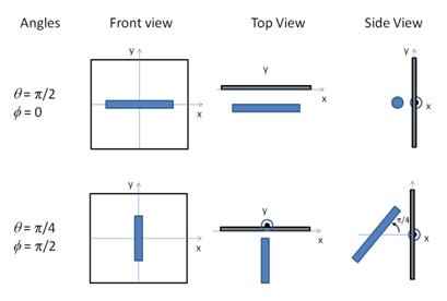
Figure 2b. Examples of the angles for oriented cylinders against the detector plane.
For P*S: The 2nd virial coefficient of the cylinder is calculate based on the radius and length values, and used as the effective radius toward S(Q) when P(Q)*S(Q) is applied.
The returned value is scaled to units of [cm-1] and the parameters of the cylinder model are the following:
|
Parameter name |
Units |
Default value |
|
scale |
None |
1.0 |
|
radius |
Å |
20.0 |
|
length |
Å |
400.0 |
|
contrast |
Å -2 |
3.0e-6 |
|
background |
cm-1 |
0.0 |
|
cyl_theta |
Radian |
1.0 |
|
cyl_phi |
Radian |
1.0 |
The output of the 1D scattering intensity function for randomly oriented cylinders is then given by:
The cyl_theta and cyl_phi parameter are not used for the 1D output. Our implementation of the scattering kernel and the 1D scattering intensity use the c-library from NIST.
2.1. Validation of the cylinder model
Validation of our code was done by comparing the output of the 1D model to the output of the software provided by the NIST (Kline, 2006). Figure 3 shows a comparison of the 1D output of our model and the output of the NIST software.
In general, averaging over a distribution of orientations is done by evaluating the following:

where p(θ,φ) is the probability distribution for the orientation and P0(q,α) is the scattering intensity for the fully oriented system. Since we have no other software to compare the implementation of the intensity for fully oriented cylinders, we can compare the result of averaging our 2D output using a uniform distribution p(θ,φ) = 1.0. Figure 4 shows the result of such a cross-check.
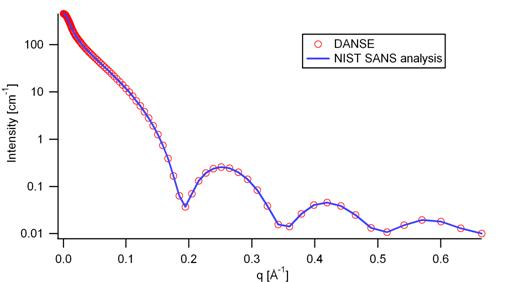
Figure 3: Comparison of the DANSE scattering intensity for a cylinder with the output of the NIST SANS analysis software. The parameters were set to: Scale=1.0, Radius=20 Å, Length=400 Å, Contrast=3e-6 Å -2, and Background=0.01 cm -1.

Figure 4: Comparison of the intensity for uniformly distributed cylinders calculated from our 2D model and the intensity from the NIST SANS analysis software. The parameters used were: Scale=1.0, Radius=20 Å, Length=400 Å, Contrast=3e-6 Å -2, and Background=0.0 cm -1.
2.9. Core-Shell Cylinder Model
This model provides the form factor for a circular cylinder with a core-shell scattering length density profile. The form factor is normalized by the particle volume.
1.1. Definition
The output of the 2D scattering intensity function for oriented core-shell cylinders is given by (Kline, 2006):
![]()

where α is the angle between the axis of the cylinder and the q-vector, Vs is the volume of the outer shell, Vc is the volume of the core, L is the length of the core, r is the radius of the core, t is the thickness of the shell, ρc is the scattering length density of the core, ρs is the scattering length density of the shell, ρsolv is the scattering length density of the solvent, and bkg is the background level. The outer radius of the shell is given by r+t and the total length of the outer shell is given by L+2t. J1 is the first order Bessel function.
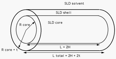
To provide easy access to the orientation of the core-shell cylinder, we define the axis of the cylinder using two angles θ and φ. Similarly to the case of the cylinder, those angles are defined on Figure 2 in Cylinder Model.
For P*S: The 2nd virial coefficient of the solid cylinder is calculate based on the (radius+thickness) and 2(length +thickness) values, and used as the effective radius toward S(Q) when P(Q)*S(Q) is applied.
The returned value is scaled to units of [cm-1] and the parameters of the core-shell cylinder model are the following:
|
Parameter name |
Units |
Default value |
|
scale |
None |
1.0 |
|
radius |
Å |
20.0 |
|
thickness |
Å |
10.0 |
|
length |
Å |
400.0 |
|
core_sld |
Å -2 |
1e-6 |
|
shell_sld |
Å -2 |
4e-6 |
|
solvent_sld |
Å -2 |
1e-6 |
|
background |
cm-1 |
0.0 |
|
axis_theta |
Radian |
1.57 |
|
axis_phi |
Radian |
0.0 |
The output of the 1D scattering intensity function for randomly oriented cylinders is then given by the equation above.
The axis_theta and axis_phi parameters are not used for the 1D output. Our implementation of the scattering kernel and the 1D scattering intensity use the c-library from NIST.
2.1. Validation of the core-shell cylinder model
Validation of our code was done by comparing the output of the 1D model to the output of the software provided by the NIST (Kline, 2006). Figure 8 shows a comparison of the 1D output of our model and the output of the NIST software.
Averaging over a distribution of orientation is done by evaluating the equation above. Since we have no other software to compare the implementation of the intensity for fully oriented core-shell cylinders, we can compare the result of averaging our 2D output using a uniform distribution p(θ,φ) = 1.0. Figure 9 shows the result of such a cross-check.

Figure 8: Comparison of the DANSE scattering intensity for a core-shell cylinder with the output of the NIST SANS analysis software. The parameters were set to: Scale=1.0, Radius=20 Å, Thickness=10 Å, Length=400 Å, Core_sld=1e-6 Å -2, Shell_sld=4e-6 Å -2, Solvent_sld=1e-6 Å -2, and Background=0.01 cm -1.

Figure 9: Comparison of the intensity for uniformly distributed core-shell cylinders calculated from our 2D model and the intensity from the NIST SANS analysis software. The parameters used were: Scale=1.0, Radius=20 Å, Thickness=10 Å, Length=400 Å, Core_sld=1e-6 Å -2, Shell_sld=4e-6 Å -2, Solvent_sld=1e-6 Å -2, and Background=0.0 cm -1.
2.10. HollowCylinderModel
This model provides the form factor, P(q), for a monodisperse hollow right angle circular cylinder (tube) where the form factor is normalized by the volume of the tube:
P(q) = scale*<f^2>/Vshell+background where the averaging < > id applied only for the 1D calculation. The inside and outside of the hollow cylinder have the same SLD.
The 1D scattering intensity is calculated in the following way (Guinier, 1955):

where scale is a scale factor, J1 is the 1st order Bessel function, J1 (x)= (sinx - xcosx)/x2.
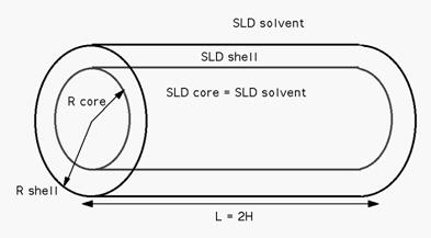
To provide easy access to the orientation of the core-shell cylinder, we define the axis of the cylinder using two angles θ and φ. Similarly to the case of the cylinder, those angles are defined on Figure 2 in Cylinder Model.
For P*S: The 2nd virial coefficient of the solid cylinder is calculate based on the (radius) and 2(length) values, and used as the effective radius toward S(Q) when P(Q)*S(Q) is applied.
In the parameters, the ‘contrast’ represents SLD (shell) - SLD (solvent) and the radius = Rhell while core_radius = Rcore.
|
Parameter name |
Units |
Default value |
|
scale |
None |
1.0 |
|
radius |
Å |
30 |
|
length |
Å |
400 |
|
core_radius |
Å |
20 |
|
sldCyl |
Å -2 |
6.3e-6 |
|
sldSolv |
Å -2 |
5e-06 |
|
background |
cm-1 |
0.01 |

Figure. 1D plot using the default values (w/1000 data point).
Our model uses the form factor calculations implemented in a c-library provided by the NIST Center for Neutron Research (Kline, 2006).
REFERENCE
Feigin, L. A, and D. I. Svergun, "Structure Analysis by Small-Angle X-Ray and Neutron Scattering", Plenum Press, New York, (1987).
This model provides the form factor, P(q), for a
flexible cylinder where the form factor is normalized by the volume of the
cylinder: Inter-cylinder interactions are NOT included. P(q) =
scale*<f^2>/V+background where the averaging < > is applied
over all orientation for 1D. The 2D scattering intensity is the same as
1D, regardless of the orientation of the q vector which is defined as![]() .
.
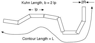
The chain of contour length, L, (the total length) can be described a chain of some number of locally stiff segments of length lp. The persistence length,lp, is the length along the cylinder over which the flexible cylinder can be considered a rigid rod. The Kuhn length (b = 2*lp) is also used to describe the stiffness of a chain. The returned value is in units of [cm-1], on absolute scale. In the parameters, the sldCyl and sldSolv represent SLD (chain/cylinder) and SLD (solvent) respectively.
|
Parameter name |
Units |
Default value |
|
scale |
None |
1.0 |
|
radius |
Å |
20 |
|
length |
Å |
1000 |
|
sldCyl |
Å -2 |
1e-06 |
|
sldSolv |
Å -2 |
6.3e-06 |
|
background |
cm-1 |
0.01 |
|
kuhn_length |
Å |
100 |

Figure. 1D plot using the default values (w/1000 data point).
Our model uses the form factor calculations implemented in a c-library provided by the NIST Center for Neutron Research (Kline, 2006):
From the reference, "Method 3 With Excluded Volume" is used. The model is a parametrization of simulations of a discrete representation of the worm-like chain model of Kratky and Porod applied in the pseudocontinuous limit. See equations (13,26-27) in the original reference for the details.
REFERENCE
Pedersen, J. S. and P. Schurtenberger (1996). “Scattering functions of semiflexible polymers with and without excluded volume effects.” Macromolecules 29: 7602-7612.
Correction of the formula can be found in:
Wei-Ren Chen, Paul D. Butler, and Linda J. Magid, "Incorporating Intermicellar Interactions in the Fitting of SANS Data from Cationic Wormlike Micelles" Langmuir, August 2006.
2.12. FlexCylEllipXModel
Flexible Cylinder with Elliptical Cross-Section: Calculates the form factor for a flexible cylinder with an elliptical cross section and a uniform scattering length density. The non-negligible diameter of the cylinder is included by accounting for excluded volume interactions within the walk of a single cylinder. The form factor is normalized by the particle volume such that P(q) = scale*<f^2>/Vol + bkg, where < > is an average over all possible orientations of the flexible cylinder.
1.1. Definition
The function calculated is from the reference given below. From that paper, "Method 3 With Excluded Volume" is used. The model is a parameterization of simulations of a discrete representation of the worm-like chain model of Kratky and Porod applied in the pseudo-continuous limit. See equations (13, 26-27) in the original reference for the details.
NOTE: there are several typos in the original reference that have been corrected by WRC. Details of the corrections are in the reference below.
- Equation (13): the term (1-w(QR)) should swap position with w(QR)
- Equations (23) and (24) are incorrect. WRC has entered these into Mathematica and solved analytically. The results were converted to code.
- Equation (27) should be q0 = max(a3/sqrt(RgSquare),3) instead of max(a3*b/sqrt(RgSquare),3)
- The scattering function is negative for a range of parameter values and q-values that are experimentally accessible. A correction function has been added to give the proper behavior.

The chain of contour length, L, (the total length) can be described a chain of some number of locally stiff segments of length lp. The persistence length, lp, is the length along the cylinder over which the flexible cylinder can be considered a rigid rod. The Kuhn length (b) used in the model is also used to describe the stiffness of a chain, and is simply b = 2*lp.
The cross section of the cylinder is elliptical, with minor radius a. The major radius is larger, so of course, the 'axis_ratio' must be greater than one. Simple constraints should be applied during curve fitting to maintain this inequality.
The returned value is in units of [cm-1], on absolute scale.
The sldCyl = SLD (chain), sldSolv = SLD (solvent). The ‘scale’, and the contrast are both multiplicative factors in the model and are perfectly correlated. One or both of these parameters must be held fixed during model fitting.
If the ‘scale’ is set equal to the particle volume fraction, f, the returned value is the scattered intensity per unit volume, I(q) = f*P(q). However, no inter-particle interference effects are included in this calculation.
For 2D data: The 2D scattering intensity is calculated in
the same way as 1D, where the q vector is defined as![]() .
.
REFERENCE
Pedersen, J. S. and P. Schurtenberger (1996). “Scattering functions of semiflexible polymers with and without excluded volume effects.” Macromolecules 29: 7602-7612.
Corrections are in:
Wei-Ren Chen, Paul D. Butler, and Linda J. Magid, "Incorporating Intermicellar Interactions in the Fitting of SANS Data from Cationic Wormlike Micelles" Langmuir, August 2006.
TEST DATASET
This example dataset is produced by running the Macro FlexCylEllipXModel, using 200 data points, qmin = 0.001 Å-1, qmax = 0.7 Å-1 and the default values below.
|
Parameter name |
Units |
Default value |
|
axis_ratio |
1.5 |
|
|
background |
cm-1 |
0.0001 |
|
Kuhn_length |
Å |
100 |
|
(Contour) length |
Å |
1e+3 |
|
radius |
Å |
20.0 |
|
scale |
1.0 |
|
|
sldCyl |
Å -2 |
1e-6 |
|
sldSolv |
Å -2 |
6.3e-6 |
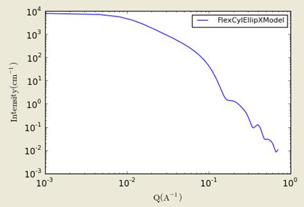
Figure. 1D plot using the default values (w/200 data point).
2.13. StackedDisksModel
This model provides the form factor, P(q), for stacked discs (tactoids) with a core/layer structure where the form factor is normalized by the volume of the cylinder. Assuming the next neighbor distance (d-spacing) in a stack of parallel discs obeys a Gaussian distribution, a structure factor S(q) proposed by Kratky and Porod in 1949 is used in this function. Note that the resolution smearing calculation uses 76 Gauss quadrature points to properly smear the model since the function is HIGHLY oscillatory, especially around the q-values that correspond to the repeat distance of the layers.
The 2D scattering intensity is the same as 1D, regardless of
the orientation of the q vector which is defined as![]() .
.


The returned value is in units of [cm-1 sr-1], on absolute scale.
The scattering intensity I(q) is:
![]()
where the contrast,
![]()
N is the number of discs per unit volume, a is the angle between the axis of the disc and q, and Vt and Vc are the total volume and the core volume of a single disc, respectively.

where d = thickness of the layer (layer_thick), 2h= core thickness (core_thick), and R = radius of the disc (radius).
![]()
where n = the total number of the disc stacked (n_stacking), D=the next neighbor center to cent distance (d-spacing), and sD = the Gaussian standard deviation of the d-spacing (sigma_d).
To provide easy access to the orientation of the stackeddisks, we define the axis of the cylinder using two angles θ and φ. Similarly to the case of the cylinder, those angles are defined on Figure 2 of CylinderModel.
For P*S: The 2nd virial coefficient of the solid cylinder is calculate based on the (radius) and length = n_stacking*(core_thick +2*layer_thick) values, and used as the effective radius toward S(Q) when P(Q)*S(Q) is applied.
|
Parameter name |
Units |
Default value |
|
background |
cm-1 |
0.001 |
|
core_sld |
Å -2 |
4e-006 |
|
core_thick |
Å |
10 |
|
layer_sld |
Å -2 |
0 |
|
layer_thick |
Å |
15 |
|
n_stacking |
|
1 |
|
radius |
Å |
3e+003 |
|
scale |
|
0.01 |
|
sigma_d |
|
0 |
|
solvent_sld |
Å -2 |
5e-006 |

Figure. 1D plot using the default values (w/1000 data point).

Figure. Examples of the angles for oriented stackeddisks against the detector plane.
Our model uses the form factor calculations implemented in a c-library provided by the NIST Center for Neutron Research (Kline, 2006):
REFERENCE
Guinier, A. and Fournet, G., "Small-Angle Scattering of X-Rays", John Wiley and Sons, New York, 1955.
Kratky, O. and Porod, G., J. Colloid Science, 4, 35, 1949.
Higgins, J.S. and Benoit, H.C., "Polymers and Neutron Scattering", Clarendon, Oxford, 1994.
2.14. ParallelepipedModel
This model provides the form factor, P(q), for a rectangular cylinder (below) where the form factor is normalized by the volume of the cylinder. P(q) = scale*<f^2>/V+background where the volume V= ABC and the averaging < > is applied over all orientation for 1D.
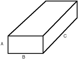
The side of the solid must be satisfied the condition of A<B<C in order for the calculation to be correct: where A = short_a, B=short_b, and C=long_c for the fitting parameters.
By this definition, assuming
a = A/B<1; b=B/B=1; c=C/B>1, the form factor,

The contrast is defined as
![]()
The scattering intensity per unit volume is returned in the unit of [cm-1]; I(q) = fP(q).
For P*S: The 2nd virial coefficient of the solid cylinder is calculate based on the averaged radius (= sqrt(short_a*short_b/pi)) and length( = long_c) values, and used as the effective radius toward S(Q) when P(Q)*S(Q) is applied.
To provide easy access to the orientation of the parallelepiped, we define the axis of the cylinder using two angles θ , φ and Y . Similarly to the case of the cylinder, those angles, θ and φ, are defined on Figure 2 of CylinderModel. The angle Y is the rotational angle around its own long_c axis against the q plane. For example, Y = 0 when the short_b axis is parallel to the x-axis of the detector.

Figure. Definition of angels for 2D.

Figure. Examples of the angles for oriented elliptical cylinders against the detector plane.
|
Parameter name |
Units |
Default value |
|
background |
cm-1 |
0.0 |
|
contrast |
Å -2 |
5e-006 |
|
long_c |
Å |
400 |
|
short_a |
Å -2 |
35 |
|
short_b |
Å |
75 |
|
scale |
|
1 |
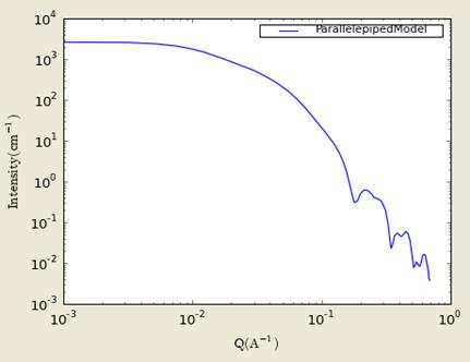
Figure. 1D plot using the default values (w/1000 data point).
· Validation of the parallelepiped 2D model
Validation of our code was done by comparing the output of the 1D calculation to the angular average of the output of 2 D calculation over all possible angles. The Figure below shows the comparison where the solid dot refers to averaged 2D while the line represents the result of 1D calculation (for the averaging, 76, 180, 76 points are taken over the angles of theta, phi, and psi respectively).
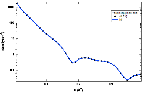
Figure. Comparison between 1D and averaged 2D.
Our model uses the form factor calculations implemented in a c-library provided by the NIST Center for Neutron Research (Kline, 2006):
REFERENCE
Mittelbach and Porod, Acta Physica Austriaca 14 (1961) 185-211.
Equations (1), (13-14). (in German)
2.15. Elliptical Cylinder Model
This function calculates the scattering from an oriented elliptical cylinder.
For 2D (orientated system):
The angles theta and phi define the orientation of the axis of the cylinder. The angle psi is defined as the orientation of the major axis of the ellipse with respect to the vector Q. A gaussian poydispersity can be added to any of the orientation angles, and also for the minor radius and the ratio of the ellipse radii.

Figure. a= r_minor and n= r_ratio (i.e., r_major/r_minor).
The function calculated is:
![]()
with the functions:
 (13)
(13)
and the angle psi is defined as the orientation of the major axis of the ellipse with respect to the vector Q.
For 1D (no preferred orientation):
The form factor is averaged over all possible orientation before normalized by the particle volume: P(q) = scale*<f^2>/V .
The returned value is scaled to units of [cm-1].
To provide easy access to the orientation of the elliptical, we define the axis of the cylinder using two angles θ , φ and Y . Similarly to the case of the cylinder, those angles, θ and φ, are defined on Figure 2 of CylinderModel. The angle Y is the rotational angle around its own long_c axis against the q plane. For example, Y = 0 when the r_minor axis is parallel to the x-axis of the detector.
All angle parameters are valid and given only for 2D calculation (Oriented system).

Figure. Definition of angels for 2D.

Figure. Examples of the angles for oriented elliptical cylinders
against the detector plane.
For P*S: The 2nd virial coefficient of the solid cylinder is calculate based on the averaged radius (=sqrt(r_minor^2*r_ratio)) and length values, and used as the effective radius toward S(Q) when P(Q)*S(Q) is applied.
|
Parameter name |
Units |
Default value |
|
scale |
None |
1.0 |
|
r_minor |
Å |
20.0 |
|
r_ratio |
Å |
1.5 |
|
length |
Å |
400.0 |
|
contrast |
Å -2 |
3e-6 |
|
cyl_phi |
Å -2 |
0 |
|
cyl_psi |
Å -2 |
0 |
|
cyl_theta |
radian |
1.57 |
|
background |
|
0 |

Figure. 1D plot using the default values (w/1000 data point).
· Validation of the elliptical cylinder 2D model
Validation of our code was done by comparing the output of the 1D calculation to the angular average of the output of 2 D calculation over all possible angles. The Figure below shows the comparison where the solid dot refers to averaged 2D while the line represents the result of 1D calculation (for 2D averaging, 76, 180, 76 points are taken for the angles of theta, phi, and psi respectively).

Figure. Comparison between 1D and averaged 2D.
In the 2D average, more binning in the angle phi is necessary to get the proper result. The following figure shows the results of the averaging by varying the number of bin over angles.

Figure. The intensities averaged from 2D over different number
of points of binning of angles.
REFERENCE
L. A. Feigin and D. I. Svergun “Structure Analysis by Small-Angle X-Ray and Neutron Scattering”, Plenum, New York, (1987).
2.16. Ellipsoid Model
This model provides the form factor for an ellipsoid (ellipsoid of revolution) with uniform scattering length density. The form factor is normalized by the particle volume.
1.1. Definition
The output of the 2D scattering intensity function for oriented ellipsoids is given by (Feigin, 1987):
![]()
![]()
![]()
where α is the angle between the axis of the ellipsoid and the q-vector, V is the volume of the ellipsoid, Ra is the radius along the rotation axis of the ellipsoid, Rb is the radius perpendicular to the rotation axis of the ellipsoid and Δρ (contrast) is the scattering length density difference between the scatterer and the solvent.
To provide easy access to the orientation of the ellipsoid, we define the rotation axis of the ellipsoid using two angles θ and φ. Similarly to the case of the cylinder, those angles are defined on Figure 2. For the ellipsoid, θ is the angle between the rotation axis and the z-axis.
For P*S: The 2nd virial coefficient of the solid ellipsoid is calculate based on the radius_a and radius_b values, and used as the effective radius toward S(Q) when P(Q)*S(Q) is applied.
The returned value is scaled to units of [cm-1] and the parameters of the ellipsoid model are the following:
|
Parameter name |
Units |
Default value |
|
scale |
None |
1.0 |
|
radius_a (polar) |
Å |
20.0 |
|
radius_b (equatorial) |
Å |
400.0 |
|
sldEll |
Å -2 |
4.0e-6 |
|
sldSolv |
Å -2 |
1.0e-6 |
|
background |
cm-1 |
0.0 |
|
axis_theta |
Radian |
1.57 |
|
axis_phi |
Radian |
0.0 |
The output of the 1D scattering intensity function for randomly oriented ellipsoids is then given by the equation above.
The axis_theta and axis_phi parameters are not used for the 1D output. Our implementation of the scattering kernel and the 1D scattering intensity use the c-library from NIST.

Figure. Examples of the angles for oriented ellipsoid
against the detector plane.
2.1. Validation of the ellipsoid model
Validation of our code was done by comparing the output of the 1D model to the output of the software provided by the NIST (Kline, 2006). Figure 5 shows a comparison of the 1D output of our model and the output of the NIST software.
Averaging over a distribution of orientation is done by evaluating the equation above. Since we have no other software to compare the implementation of the intensity for fully oriented ellipsoids, we can compare the result of averaging our 2D output using a uniform distribution p(θ,φ) = 1.0. Figure 6 shows the result of such a cross-check.
The discrepancy above q=0.3 Å -1 is due to the way the form factors are calculated in the c-library provided by NIST. A numerical integration has to be performed to obtain P(q) for randomly oriented particles. The NIST software performs that integration with a 76-point Gaussian quadrature rule, which will become imprecise at high q where the amplitude varies quickly as a function of q. The DANSE result shown has been obtained by summing over 501 equidistant points in α. Our result was found to be stable over the range of q shown for a number of points higher than 500.

Figure 5: Comparison of the DANSE scattering intensity for an ellipsoid with the output of the NIST SANS analysis software. The parameters were set to: Scale=1.0, Radius_a=20 Å, Radius_b=400 Å,
Contrast=3e-6 Å -2, and Background=0.01 cm -1.
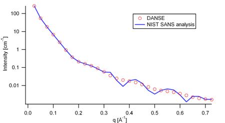
Figure 6: Comparison of the intensity for uniformly distributed ellipsoids calculated from our 2D model and the intensity from the NIST SANS analysis software. The parameters used were: Scale=1.0, Radius_a=20 Å, Radius_b=400 Å, Contrast=3e-6 Å -2, and Background=0.0 cm -1.
2.17. CoreShellEllipsoidModel
This model provides the form factor, P(q), for a core shell ellipsoid (below) where the form factor is normalized by the volume of the cylinder. P(q) = scale*<f^2>/V+background where the volume V= 4pi/3*rmaj*rmin2 and the averaging < > is applied over all orientation for 1D.
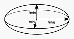
The returned value is in units of [cm-1], on absolute scale.
The form factor calculated is:

To provide easy access to the orientation of the coreshell ellipsoid, we define the axis of the solid ellipsoid using two angles θ , φ. Similarly to the case of the cylinder, those angles, θ and φ, are defined on Figure 2 of CylinderModel.
The contrast is defined as SLD(core) – SLD(shell) or SLD(shell – solvent). In the parameters, equat_core = equatorial radius of the core, polar_core = polar radius of the core, equat_shell = rmin (or equatorial radius of the shell), and polar_shell = = rmaj (or polar radius of the shell).
For P*S: The 2nd virial coefficient of the solid ellipsoid is calculate based on the radius_a (= polar_shell) and radius_b (= equat_shell) values, and used as the effective radius toward S(Q) when P(Q)*S(Q) is applied.
|
Parameter name |
Units |
Default value |
|
background |
cm-1 |
0.001 |
|
equat_core |
Å |
200 |
|
equat_shell |
Å |
250 |
|
sld_solvent |
Å -2 |
6e-006 |
|
ploar_shell |
Å |
30 |
|
ploar_core |
Å |
20 |
|
scale |
|
1 |
|
sld_core |
Å -2 |
2e-006 |
|
sld_shell |
Å -2 |
1e-006 |
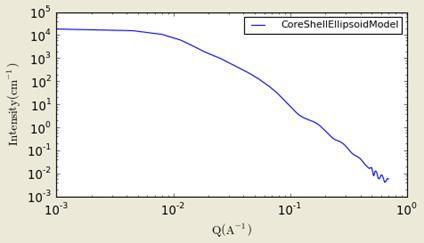
Figure. 1D plot using the default values (w/1000 data point).

Figure. Examples of the angles for oriented coreshellellipsoid against the detector plane where a =polar axis.
Our model uses the form factor calculations implemented in a c-library provided by the NIST Center for Neutron Research (Kline, 2006):
REFERENCE
Kotlarchyk, M.; Chen, S.-H. J. Chem. Phys., 1983, 79, 2461.
Berr, S. J. Phys. Chem., 1987, 91, 4760.
2.18. TriaxialEllipsoidModel
This model provides the form factor, P(q), for an ellipsoid (below) where all three axes are of different lengths, i.e., Ra =< Rb =< Rc (Note that users should maintains this inequality for the all calculations). P(q) = scale*<f^2>/V+background where the volume V= 4pi/3*Ra*Rb*Rc, and the averaging < > is applied over all orientation for 1D.

The returned value is in units of [cm-1], on absolute scale.
The form factor calculated is:

To provide easy access to the orientation of the triaxial ellipsoid, we define the axis of the cylinder using the angles θ , φ and Y . Similarly to the case of the cylinder, those angles, θ and φ, are defined on Figure 2 of CylinderModel. The angle Y is the rotational angle around its own semi_axisC axis against the q plane. For example, Y = 0 when the semi_axisA axis is parallel to the x-axis of the detector.
The radius of gyration for this system is Rg2 = (Ra2*Rb2*Rc2)/5. The contrast is defined as SLD(ellipsoid) – SLD(solvent). In the parameters, semi_axisA = Ra (or minor equatorial radius), semi_axisB = Rb (or major equatorial radius), and semi_axisC = Rc (or polar radius of the ellipsoid).
For P*S: The 2nd virial coefficient of the solid ellipsoid is calculate based on the radius_a (=semi_axisC) and radius_b (=sqrt(semi_axisA* semi_axisB)) values, and used as the effective radius toward S(Q) when P(Q)*S(Q) is applied.
|
Parameter name |
Units |
Default value |
|
background |
cm-1 |
0.0 |
|
semi_axisA |
Å |
35 |
|
semi_axisB |
Å |
100 |
|
semi_axisC |
Å |
400 |
|
scale |
|
1 |
|
sldEll |
Å -2 |
1.0e-006 |
|
sldSolv |
Å -2 |
6.3e-006 |
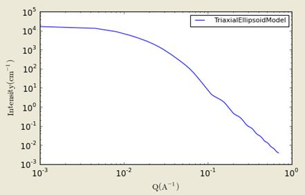
Figure. 1D plot using the default values (w/1000 data point).
· Validation of the triaxialellipsoid 2D model
Validation of our code was done by comparing the output of the 1D calculation to the angular average of the output of 2 D calculation over all possible angles. The Figure below shows the comparison where the solid dot refers to averaged 2D while the line represents the result of 1D calculation (for 2D averaging, 76, 180, 76 points are taken for the angles of theta, phi, and psi respectively).

Figure. Comparison between 1D and averaged 2D.
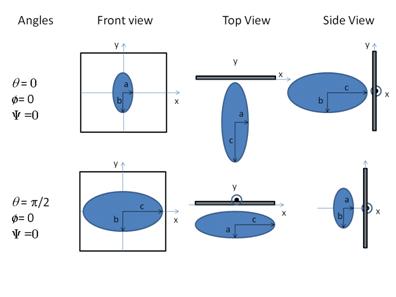
Figure. Examples of the angles for oriented ellipsoid against the detector plane.
Our model uses the form factor calculations implemented in a c-library provided by the NIST Center for Neutron Research (Kline, 2006):
REFERENCE
L. A. Feigin and D. I. Svergun “Structure Analysis by Small-Angle X-Ray and Neutron Scattering”, Plenum, New York, 1987.
2.19. LamellarModel
This model provides the scattering intensity, I(q), for a lyotropic lamellar phase where a uniform SLD and random distribution in solution are assumed. The ploydispersion in the bilayer thickness can be applied from the GUI.
The scattering intensity I(q) is:
![]()
The form factor is,
![]()
where d = bilayer thickness.
The 2D scattering intensity is calculated in the same way as
1D, where the q vector is defined as![]() .
.
The returned value is in units of [cm-1], on absolute scale. In the parameters, sld_bi = SLD of the bilayer, sld_sol = SLD of the solvent, and bi_thick = the thickness of the bilayer.
|
Parameter name |
Units |
Default value |
|
background |
cm-1 |
0.0 |
|
sld_bi |
Å -2 |
1e-006 |
|
bi_thick |
Å |
50 |
|
sld_sol |
Å -2 |
6e-006 |
|
scale |
|
1 |

Figure. 1D plot using the default values (w/1000 data point).
Our model uses the form factor calculations implemented in a c-library provided by the NIST Center for Neutron Research (Kline, 2006):
REFERENCE
Nallet, Laversanne, and Roux, J. Phys. II France, 3, (1993) 487-502.
also in J. Phys. Chem. B, 105, (2001) 11081-11088.
2.20. LamellarFFHGModel
This model provides the scattering intensity, I(q), for a lyotropic lamellar phase where a random distribution in solution are assumed. The SLD of the head region is taken to be different from the SLD of the tail region.
The scattering intensity I(q) is:
![]()
The form factor is,
![]()
where dT = tail length (or t_length), dH = heasd thickness (or h_thickness) , DrH = SLD (headgroup) - SLD(solvent), and DrT = SLD (tail) - SLD(headgroup).
The 2D scattering intensity is calculated in the same way as
1D, where the q vector is defined as![]() .
.
The returned value is in units of [cm-1], on absolute scale. In the parameters, sld_tail = SLD of the tail group, and sld_head = SLD of the head group.
|
Parameter name |
Units |
Default value |
|
background |
cm-1 |
0.0 |
|
sld_head |
Å -2 |
3e-006 |
|
scale |
|
1 |
|
sld_solvent |
Å -2 |
6e-006 |
|
h_thickness |
Å |
10 |
|
t_length |
Å |
15 |
|
sld_tail |
Å -2 |
0 |

Figure. 1D plot using the default values (w/1000 data point).
Our model uses the form factor calculations implemented in a c-library provided by the NIST Center for Neutron Research (Kline, 2006):
REFERENCE
Nallet, Laversanne, and Roux, J. Phys. II France, 3, (1993) 487-502.
also in J. Phys. Chem. B, 105, (2001) 11081-11088.
2.21. LamellarPSModel
This model provides the scattering intensity (form factor * structure factor), I(q), for a lyotropic lamellar phase where a random distribution in solution are assumed.
The scattering intensity I(q) is:
![]()
The form factor is
![]()
and the structure is

where

Here d= (repeat) spacing, d = bilayer thickness, the contrast Dr = SLD (headgroup) - SLD(solvent), K=smectic bending elasticity, B=compression modulus, and N = number of lamellar plates (n_plates).
Note: When the Caille parameter is greater than approximately 0.8 to 1.0, the assumptions of the model are incorrect. And due to the complication of the model function, users are responsible to make sure that all the assumptions are handled accurately: see the original reference (below) for more details.
The 2D scattering intensity is calculated in the same way as
1D, where the q vector is defined as![]() .
.
The returned value is in units of [cm-1], on absolute scale.
|
Parameter name |
Units |
Default value |
|
background |
cm-1 |
0.0 |
|
contrast |
Å -2 |
5e-006 |
|
scale |
|
1 |
|
delta |
Å |
30 |
|
n_plates |
|
20 |
|
spacing |
Å |
400 |
|
caille |
Å -2 |
0.1 |
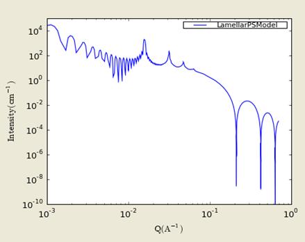
Figure. 1D plot using the default values (w/6000 data point).
Our model uses the form factor calculations implemented in a c-library provided by the NIST Center for Neutron Research (Kline, 2006):
REFERENCE
Nallet, Laversanne, and Roux, J. Phys. II France, 3, (1993) 487-502.
also in J. Phys. Chem. B, 105, (2001) 11081-11088.
2.22. LamellarPSHGModel
This model provides the scattering intensity (form factor * structure factor), I(q), for a lyotropic lamellar phase where a random distribution in solution are assumed. The SLD of the head region is taken to be different from the SLD of the tail region.
The scattering intensity I(q) is:
![]()
The form factor is,
![]()
The structure factor is

where

where dT = tail length (or t_length), dH = heasd thickness (or h_thickness) , DrH = SLD (headgroup) - SLD(solvent), and DrT = SLD (tail) - SLD(headgroup). Here d= (repeat) spacing, K=smectic bending elasticity, B=compression modulus, and N = number of lamellar plates (n_plates).
Note: When the Caille parameter is greater than approximately 0.8 to 1.0, the assumptions of the model are incorrect. And due to the complication of the model function, users are responsible to make sure that all the assumptions are handled accurately: see the original reference (below) for more details.
The 2D scattering intensity is calculated in the same way as
1D, where the q vector is defined as![]() .
.
The returned value is in units of [cm-1], on absolute scale. In the parameters, sld_tail = SLD of the tail group, sld_head = SLD of the head group, and sld_solvent = SLD of the solvent.
|
Parameter name |
Units |
Default value |
|
background |
cm-1 |
0.001 |
|
sld_head |
Å -2 |
2e-006 |
|
scale |
|
1 |
|
sld_solvent |
Å -2 |
6e-006 |
|
deltaH |
Å |
2 |
|
deltaT |
Å |
10 |
|
sld_tail |
Å -2 |
0 |
|
n_plates |
|
30 |
|
spacing |
Å |
40 |
|
caille |
Å -2 |
0.001 |

Figure. 1D plot using the default values (w/6000 data point).
Our model uses the form factor calculations implemented in a c-library provided by the NIST Center for Neutron Research (Kline, 2006):
REFERENCE
Nallet, Laversanne, and Roux, J. Phys. II France, 3, (1993) 487-502.
also in J. Phys. Chem. B, 105, (2001) 11081-11088.
The following are models used for shape-independent SANS analysis.
3.1. Debye (Model)
The Debye model is a form factor for a linear polymer chain. In addition to the radius of gyration, Rg, a scale factor "scale", and a constant background term are included in the calculation.

For 2D plot, the wave transfer is defined
as ![]() .
.
|
Parameter name |
Units |
Default value |
|
scale |
None |
1.0 |
|
rg |
Å |
50.0 |
|
background |
cm-1 |
0.0 |

Figure. 1D plot using the default values (w/200 data point).
Reference: Roe, R.-J., "Methods of X-Ray and Neutron Scattering in Polymer Science", Oxford University Press, New York (2000).
3.2. (Ornstein-Zernicke) Lorentz (Model)
The Ornstein-Zernicke model is defined by:
![]()
The parameter L is referred to as the screening length.
For 2D plot, the wave transfer is
defined as ![]() .
.
|
Parameter name |
Units |
Default value |
|
scale |
None |
1.0 |
|
length |
Å |
50.0 |
|
background |
cm-1 |
0.0 |

Figure. 1D plot using the default values (w/200 data point).
3.3. DAB (Debye-Anderson-Brumberger)_Model
Calculates the scattering from a randomly distributed, two-phase system based on the Debye-Anderson-Brumberger (DAB) model for such systems. The two-phase system is characterized by a single length scale, the correlation length, which is a measure of the average spacing between regions of phase 1 and phase 2. The model also assumes smooth interfaces between the phases and hence exhibits Porod behavior (I ~ Q-4) at large Q (Q*correlation length >> 1).
![]()
The parameter L is referred to as the correlation length.
For 2D plot, the wave transfer is
defined as ![]() .
.
|
Parameter name |
Units |
Default value |
|
scale |
None |
1.0 |
|
length |
Å |
50.0 |
|
background |
cm-1 |
0.0 |
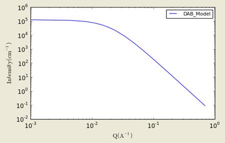
Figure. 1D plot using the default values (w/200 data point).
References:
Debye, Anderson, Brumberger, "Scattering by an Inhomogeneous Solid. II. The Correlation Function and its Application", J. Appl. Phys. 28 (6), 679 (1957).
Debye, Bueche, "Scattering by an Inhomogeneous Solid", J. Appl. Phys. 20, 518 (1949).
3.4. Power_Law
This model describes a power law with background.
![]()
Note the minus sign in front of the exponent.
|
Parameter name |
Units |
Default value |
|
Scale |
None |
1.0 |
|
m |
None |
4 |
|
Background |
cm-1 |
0.0 |

Figure. 1D plot using the default values (w/200 data point).
This function calculates the scattered intensity of a two-component system using the Teubner-Strey model.
![]()
For 2D plot, the wave transfer is
defined as ![]() .
.
|
Parameter name |
Units |
Default value |
|
scale |
None |
0.1 |
|
c1 |
None |
-30.0 |
|
c2 |
None |
5000.0 |
|
background |
cm-1 |
0.0 |
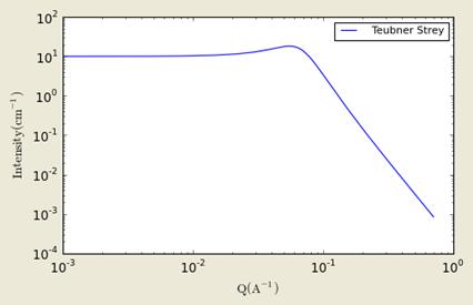
Figure. 1D plot using the default values (w/200 data point).
References:
Teubner, M; Strey, R. J. Chem. Phys., 87, 3195 (1987).
Schubert, K-V., Strey, R., Kline, S. R. and E. W. Kaler, J. Chem. Phys., 101, 5343 (1994).
3.6. FractalModel
Calculates the scattering from fractal-like aggregates built from spherical building blocks following the Texiera reference. The value returned is in cm-1.

The scale parameter is the volume fraction of the building blocks, R0 is the radius of the building block, Df is the fractal dimension, ξ is the correlation length, ρsolvent is the scattering length density of the solvent, and ρblock is the scattering length density of the building blocks.
The polydispersion in radius is provided.
For 2D plot, the wave transfer is
defined as ![]() .
.
|
Parameter name |
Units |
Default value |
|
scale |
None |
0.05 |
|
radius |
Å |
5.0 |
|
fractal_dim |
None |
2 |
|
corr_length |
Å |
100.0 |
|
block_sld |
Å-2 |
2e-6 |
|
solvent_sld |
Å-2 |
6e-6 |
|
background |
cm-1 |
0.0 |

Figure. 1D plot using the default values (w/200 data point).
References:
J. Teixeira, (1988) J. Appl. Cryst., vol. 21, p781-785
Calculates the structure factor of a polyelectrolyte solution with the RPA expression derived by Borue and Erukhimovich. The value returned is in cm-1.

K is a contrast factor of the polymer, Lb is the Bjerrum length, h is the virial parameter, b is the monomer length, Cs is the concentration of monovalent salt, α is the ionization degree, Ca is the polymer molar concentration, and background is the incoherent background.
For 2D plot, the wave transfer is
defined as ![]() .
.
|
Parameter name |
Units |
Default value |
|
K |
Barns = 10-24 cm2 |
10 |
|
Lb |
Å |
7.1 |
|
h |
Å-3 |
12 |
|
b |
Å |
10 |
|
Cs |
Mol/L |
0 |
|
alpha |
None |
0.05 |
|
Ca |
Mol/L |
0.7 |
|
background |
cm-1 |
0.0 |
References:
Borue, V. Y., Erukhimovich, I. Y. Macromolecules 21, 3240 (1988).
Joanny, J.-F., Leibler, L. Journal de Physique 51, 545 (1990).
Moussaid, A., Schosseler, F., Munch, J.-P., Candau, S. J. Journal de Physique II France
3, 573 (1993).
Raphaël, E., Joanny, J.-F., Europhysics Letters 11, 179 (1990).
3.8. Guinier (Model)
A Guinier analysis is done by linearizing the data at low q by plotting it as log(I) versus Q2. The Guinier radius Rg can be obtained by fitting the following model:
![]()
For 2D plot, the wave transfer is
defined as ![]() .
.
|
Parameter name |
Units |
Default value |
|
scale |
cm-1 |
1.0 |
|
Rg |
Å |
0.1 |
3.9. PorodModel
A Porod analysis is done by linearizing the data at high q by plotting it as log(I) versus log(Q). In the high q region we can fit the following model:
![]()
C is the scale factor and Sv is the specific surface area of the sample and Δρ is the contrast factor.
The background term is added for data analysis.
For 2D plot, the wave transfer is
defined as ![]() .
.
|
Parameter name |
Units |
Default value |
|
scale |
Å-4 |
0.1 |
|
background |
cm-1 |
0 |
3.10 Poly_GaussCoil (Model)
Polydisperse Gaussian Coil: Calculate an empirical functional form for scattering from a polydisperse polymer chain ina good solvent. The polymer is polydisperse with a Schulz-Zimm polydispersity of the molecular weight distribution.
The returned value is scaled to units of [cm-1sr-1], absolute scale.
![]()
where the dimensionless chain dimension is:
![]()
and the polydispersion is
![]() .
.
The scattering intensity I(q) is calculated as:
The polydispersion in ‘rg’ is provided.
For 2D plot, the wave transfer is
defined as ![]() .
.
TEST DATASET
This example dataset is produced by running the Poly_GaussCoil, using 200 data points, qmin = 0.001 Å-1, qmax = 0.7 Å-1 and the default values below.
|
Parameter name |
Units |
Default value |
|
Scale |
None |
1.0 |
|
rg |
Å |
60.0 |
|
poly_m |
Mw/Mn |
2 |
|
background |
cm-1 |
0.001 |

Figure. 1D plot using the default values (w/200 data point).
Reference:
Glatter & Kratky - pg.404.
J.S. Higgins, and H.C. Benoit, “Polymers and Neutron Scattering”, Oxford Science
Publications (1996).
3.11. Peak Gauss Model
This Gaussian peak model with a flat background calculates:
![]()
where ‘scale’ is the peak height centered at q0, and B refers to the standard deviation of the function (equivalently, the FWHM is 2.54*B).
The background term is added for data analysis.
For 2D plot, the wave transfer is
defined as ![]() .
.
|
Parameter name |
Units |
Default value |
|
scale |
cm-1 |
100 |
|
B |
Å-1 |
0.005 |
|
q0 |
Å-1 |
0.05 |
|
background |
cm-1 |
1.0 |
3.12. Peak Lorentz Model
This Lorentzean peak model with a flat background calculates:

where ‘scale’ is the peak height centered at q0, and B refers to the standard deviation of the function.
The background term is added for data analysis.
For 2D plot, the wave transfer is
defined as![]() .
.
|
Parameter name |
Units |
Default value |
|
scale |
cm-1 |
100 |
|
B |
Å-1 |
0.005 |
|
q0 |
Å-1 |
0.05 |
|
background |
cm-1 |
1.0 |
3.13. LineModel
This is a linear function that calculates:
![]()
where A and B are the coefficients of the first and second order terms.
Note: For 2D plot, I(q) = I(qx)*I(qy) which is defined differently from other shape independent models.
|
Parameter name |
Units |
Default value |
|
A |
cm-1 |
1.0 |
|
B |
Å |
1.0 |
These model functions can be redefined by users (See SansView tutorial for details).
4.1. A+Bcos(2x)+Csin(2x)
This function, as a sample function, calculates the intensity = A + Bcos(2q) + Csin(2q).
4.2. sin(poly)/poly
This function calculates the intensity = scale * sin(f)/f, where f = A + Bq + Cq2 + Dq3 + Eq4 + Fq5.
The information in this section is originated from NIST SANS IgorPro package.
5.1. HardSphere Structure
This calculates the interparticle structure factor for monodisperse spherical particles interacting through hard sphere (excluded volume) interactions. The calculation uses the Percus-Yevick closure where the interparticle potential is:
![]()
where r is the distance from the center of the sphere of a radius R.
For 2D plot, the wave transfer is
defined as![]() .
.
|
Parameter name |
Units |
Default value |
|
effect_radius |
Å |
50.0 |
|
volfraction |
|
0.2 |
|
|
|
|

Figure. 1D plot using the default values (in linear scale).
References:
Percus, J. K.; Yevick, J. Phys. Rev. 110, 1. (1958).
5.2. SquareWell Structure
This calculates the interparticle structure factor for a squar well fluid spherical particles The mean spherical approximation (MSA) closure was used for this calculation, and is not the most appropriate closure for an attractive interparticle potential. This solution has been compared to Monte Carlo simulations for a square well fluid, showing this calculation to be limited in applicability to well depths e < 1.5 kT and volume fractions f < 0.08.
Positive well depths correspond to an attractive potential well. Negative well depths correspond to a potential "shoulder", which may or may not be physically reasonable.
The well width (l) is defined as multiples of the particle diameter (2*R)
The interaction potential is:

where r is the distance from the center of the sphere of a radius R.
For 2D plot, the wave transfer is
defined as![]() .
.
|
Parameter name |
Units |
Default value |
|
effect_radius |
Å |
50.0 |
|
volfraction |
|
0.04 |
|
welldepth |
kT |
1.5 |
|
wellwidth |
diameters |
1.2 |

Figure. 1D plot using the default values (in linear scale).
References:
Sharma, R. V.; Sharma, K. C. Physica, 89A, 213. (1977).
5.3. HayterMSA Structure
This calculates the Structure factor (the Fourier transform of the pair correlation function g(r)) for a system of charged, spheroidal objects in a dielectric medium. When combined with an appropriate form factor (such as sphere, core+shell, ellipsoid etc…), this allows for inclusion of the interparticle interference effects due to screened coulomb repulsion between charged particles. This routine only works for charged particles. If the charge is set to zero the routine will self destruct. For non-charged particles use a hard sphere potential.
The salt concentration is used to compute the ionic strength of the solution which in turn is used to compute the Debye screening length. At present there is no provision for entering the ionic strength directly nor for use of any multivalent salts. The counterions are also assumed to be monovalent.
For 2D plot, the wave transfer is
defined as![]() .
.
|
Parameter name |
Units |
Default value |
|
effect_radius |
Å |
20.8 |
|
charge |
|
19 |
|
volfraction |
|
0.2 |
|
temperature |
K |
318 |
|
salt conc |
M |
0 |
|
dielectconst |
|
71.1 |
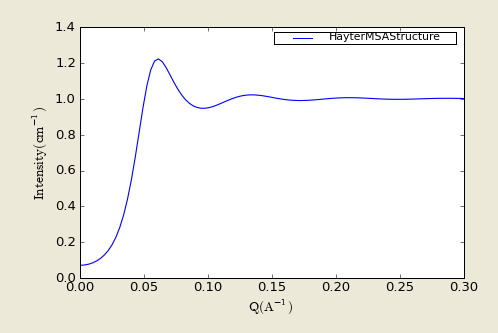
Figure. 1D plot using the default values (in linear scale).
References:
JP Hansen and JB Hayter, Molecular Physics 46, 651-656 (1982).
JB Hayter and J Penfold, Molecular Physics 42, 109-118 (1981).
5.4. StickyHS Structure
This calculates the interparticle structure factor for a hard sphere fluid with a narrow attractive well. A perturbative solution of the Percus-Yevick closure is used. The strength of the attractive well is described in terms of "stickiness" as defined below. The returned value is a dimensionless structure factor, S(q).
The perturb (perturbation parameter), epsilon, should be held between 0.01 and 0.1. It is best to hold the perturbation parameter fixed and let the "stickiness" vary to adjust the interaction strength. The stickiness, tau, is defined in the equation below and is a function of both the perturbation parameter and the interaction strength. Tau and epsilon are defined in terms of the hard sphere diameter (sigma = 2R), the width of the square well, delta (same units as R), and the depth of the well, uo, in units of kT. From the definition, it is clear that smaller tau mean stronger attraction.

where the interaction potential is

The Percus-Yevick (PY) closure was used for this calculation, and is an adequate closure for an attractive interparticle potential. This solution has been compared to Monte Carlo simulations for a square well fluid, with good agreement.
The true particle volume fraction, f, is not equal to h, which appears in most of the reference. The two are related in equation (24) of the reference. The reference also describes the relationship between this perturbation solution and the original sticky hard sphere (or adhesive sphere) model by Baxter.
NOTES: The calculation can go haywire for certain combinations of the input parameters, producing unphysical solutions - in this case errors are reported to the command window and the S(q) is set to -1 (it will disappear on a log-log plot). Use tight bounds to keep the parameters to values that you know are physical (test them) and keep nudging them until the optimization does not hit the constraints.
For 2D plot, the wave transfer is
defined as![]() .
.
|
Parameter name |
Units |
Default value |
|
effect_radius |
Å |
50 |
|
perturb |
|
0.05 |
|
volfraction |
|
0.1 |
|
stickiness |
K |
0.2 |
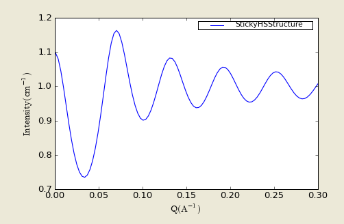
Figure. 1D plot using the default values (in linear scale).
References:
Menon, S. V. G., Manohar, C. and K. Srinivas Rao J. Chem. Phys., 95(12), 9186-9190 (1991).
Feigin, L. A, and D. I. Svergun (1987) "Structure Analysis by Small-Angle X-Ray and Neutron Scattering", Plenum Press, New York.
Guinier, A. and G. Fournet (1955) "Small-Angle Scattering of X-Rays", John Wiley and Sons, New York.
Kline, S. R. (2006) J Appl. Cryst. 39(6), 895.
Hansen, S., (1990) J. Appl. Cryst. 23, 344-346.
Henderson, S.J. (1996) Biophys. J. 70, 1618-1627
Stöckel, P., May, R., Strell, I., Cejka, Z., Hoppe, W., Heumann, H., Zillig, W. and Crespi, H. (1980) Eur. J. Biochem. 112, 411-417.
McAlister, B.C. and Grady, B.P., (1998) J. Appl. Cryst. 31, 594-599.
Porod, G. (1982) in Small Angle X-ray Scattering, editors Glatter, O. and Kratky, O., Academic Press.
*Also, see the references in the each model function descriptions.
